Type II Supernovae

Type II core-collapse supernovae (CCSNe) are the explosions of massive stars that retained at least part of their hydrogen envelope. Type IIP events are the explosions of hydrogen-rich stars: an early cooling-phase decline (from the initial shock breakout) settles onto a weeks-to-months-long luminosity “plateau” as a recombination front recedes through the ejecta, followed by a radioactive tail powered by \(^{56}\mathrm{Co}\) decay. A subset show a brighter, hotter, faster early excess on top of this, attributed to shock breakout through and/or collisional heating of close circumstellar material – IXF/GGI-like objects, after the prototypes SN 2023ixf and SN 2024ggi. Both IIP variants share the same SED functional form and differ only in their parameter priors. Type IIb events, which lost most but not all of their hydrogen, are modeled with a different, double-pulse form. Each is implemented as its own transient population in a tab below. (Hydrogen-free Type Ib and Ic supernovae are covered on the Type I page.)

Type IIP

Implemented by TypeIIPSNe, pairing TypeIIPSED with the rate/duration metadata described below.

Quick Facts

Quantity	Value	Source	Notes
Rate	\(R_\mathrm{CC}(z) = k\,\psi_\mathrm{UV}(z)\); Type IIP 48.7% of \(R_\mathrm{CC}(z)\)	Strolger et al.[1], Madau and Dickinson[2], Li et al.[3], Shivvers et al.[4]	Tracks the cosmic star-formation history. Li et al.[3] find II-P is \(69.9^{+5.1}_{-5.8}\%\) of the Type II rate, which is itself \(69.6\pm6.7\%\) of the total core-collapse rate [4], so the Type IIP fraction of the CC rate is \(0.699\times0.696=0.487\). This chain, combined in quadrature with the \(+27\%/-31\%\) uncertainty on Strolger et al.[1]’s \(k\), gives RATE_CI; see Rate Uncertainty and All-Sky Yield.
Redshift limit	\(z = 0.8\)	–	Matched to ordinary Type IIP peak luminosities.
Duration	100 days	–	Covers the plateau and the transition to the (unmodeled) nebular phase.

SED Model

TypeIIPSED is two shared-onset exponential components (an early cooling-phase decline onto a constant plateau) plus a switched radioactive tail, together with a smooth, doubly-broken power-law photospheric temperature that reuses the light curve’s own \(t_0\)/\(t_P\):

\[L_\mathrm{bol}(t) = S_0(t)\,\bigl[1-S_P(t)\bigr] \Bigl[L_\mathrm{pk}\,e^{-(t-t_0)/\tau_\mathrm{cool}} + L_p\Bigr] + S_P(t)\, L_\mathrm{Co}\, e^{-(t-t_P)/\tau_\mathrm{Co}},\]

with two logistic switches

\[S_0(t) = \frac{1}{1+e^{-(t-t_0)/\tau_\mathrm{rise}}}, \qquad S_P(t) = \frac{1}{1+e^{-(t-t_P)/\tau_\mathrm{drop}}}.\]

\(S_0\) turns the photospheric emission on at the explosion/rise epoch \(t_0\); \(S_P\) turns it back off – and the radioactive tail on – at the plateau-end epoch \(t_P\). Between the rise and \(t_P\), \(L_\mathrm{bol}\) is an early cooling-phase decline from \(L_\mathrm{pk}\) onto a constant plateau \(L_p\); after \(t_P\) it switches to a pure radioactive-tail exponential.

The temperature law has three regimes – an early regime, a cooling-phase regime around \(t_0\), and a recombination/plateau regime around \(t_P\) – joined by two smooth breaks:

\[T(t) = T_0\, \left(\frac{t}{t_0}\right)^{\alpha_r} \left(\frac{1 + (t/t_0)^{s_0}}{2}\right)^{\frac{\alpha_c - \alpha_r}{s_0}} \left(\frac{1 + (t/\sqrt{t_0 t_P})^{s_1}}{2}\right)^{-\frac{\alpha_c - \alpha_p}{s_1}},\]

with \(t\) in days, so that \(T(t_0) \approx T_0\). With \(\alpha_r > 0 > \alpha_c > \alpha_p\), the temperature rises through the early, pre-\(t_0\) region (where \(L_\mathrm{bol} \approx 0\) anyway), peaks near \(t_0\), then declines – fast through the cooling regime and much more slowly through the recombination/plateau regime. \(s_0\)/\(s_1\) set the sharpness of the two breaks. The second break has no epoch of its own, so it is centered on the geometric mean of \(t_0\) and \(t_P\).

Parameter priors

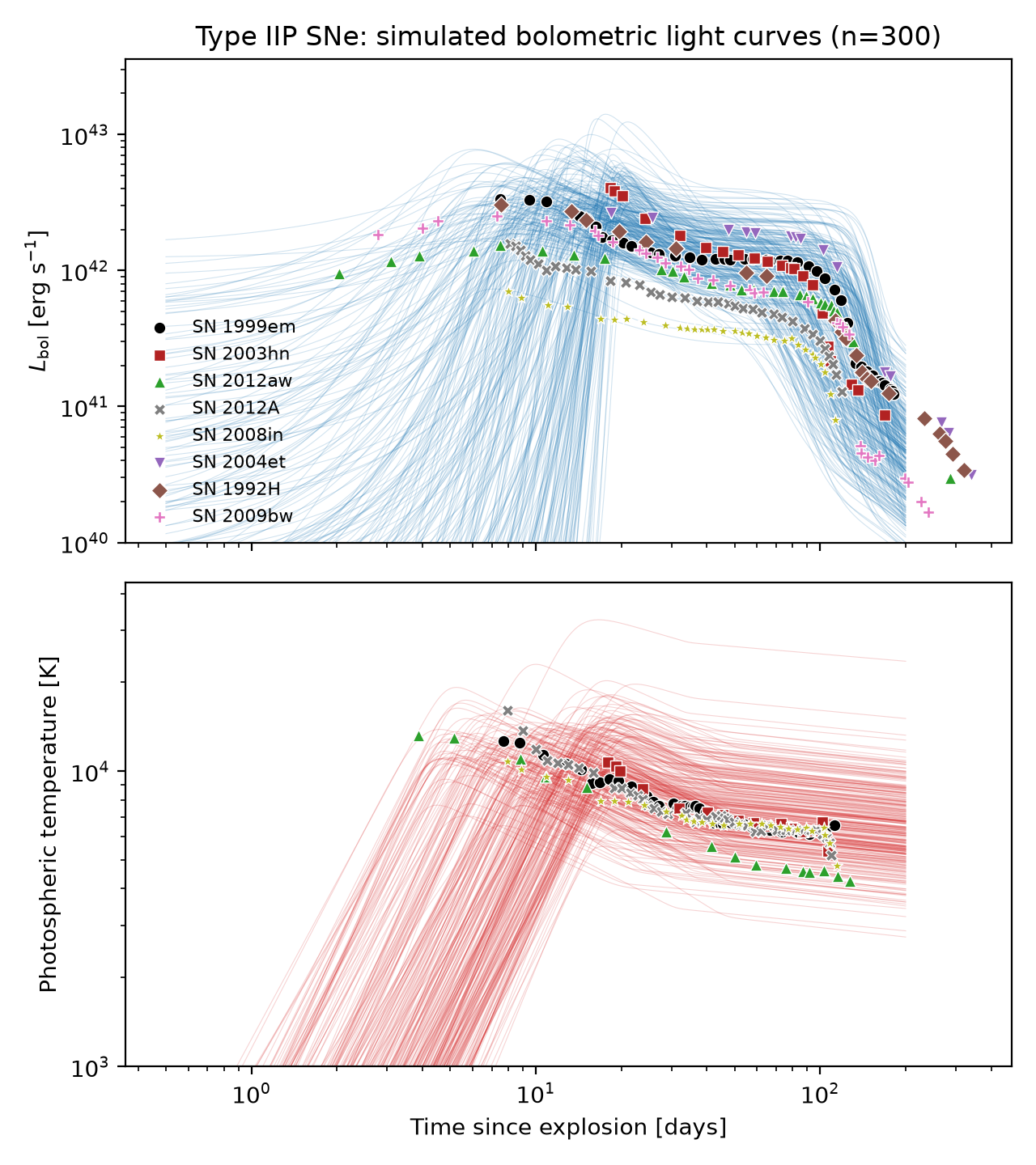
Light-curve priors (t0 through tau_Co) come from fitting the light-curve model to SN 1999em and SN 2003hn; temperature-law priors (T_0 through s_1) are hand-tuned against the aggregate Type IIP temperature dataset in the plot below.

Parameter	Symbol	Prior	Notes
t0	\(t_0\)	Uniform(4 d, 20 d)	Explosion/rise reference epoch.
tau_rise	\(\tau_\mathrm{rise}\)	Normal(\(\log_{10}(\tau_\mathrm{rise}/\mathrm{d})\); mean=0, \(\sigma\)=0.2)	Rise timescale (median 1 d).
L_pk	\(L_\mathrm{pk}\)	Normal(\(\log_{10}(L_\mathrm{pk}/\mathrm{erg\,s^{-1}})\); mean=42.48, \(\sigma\)=0.2)	Early cooling-phase peak luminosity scale (median \(\sim3\times10^{42}\) erg/s).
tau_cool	\(\tau_\mathrm{cool}\)	Uniform(4 d, 10 d)	Early cooling-phase decay timescale.
L_p	\(L_p\)	Normal(\(\log_{10}(L_p/\mathrm{erg\,s^{-1}})\); mean=42.1, \(\sigma\)=0.1)	Plateau luminosity.
t_P	\(t_P\)	Uniform(50 d, 150 d)	Plateau-end / radioactive-tail-onset epoch.
tau_drop	\(\tau_\mathrm{drop}\)	Fixed (10.5 d)	Plateau-end transition width.
L_Co	\(L_\mathrm{Co}\)	Normal(\(\log_{10}(L_\mathrm{Co}/\mathrm{erg\,s^{-1}})\); mean=41.39, \(\sigma\)=0.1)	Radioactive-tail luminosity at t_P.
tau_Co	\(\tau_\mathrm{Co}\)	Fixed (111.4 d)	Radioactive-tail decay timescale, fixed to the \(^{56}\mathrm{Co}\) e-folding time.
T_0	\(T_0\)	Normal(\(\log_{10}(T_0/\mathrm{K})\); mean=4.05, \(\sigma\)=0.1)	Normalization: \(T(t_0) \approx T_0\) (\(\sim1.1\times10^4\) K).
alpha_r	\(\alpha_r\)	Normal(2, \(\sigma\)=0.2)	Early-regime power-law index; \(T\) rises toward \(t_0\).
alpha_c	\(\alpha_c\)	Normal(-0.45, \(\sigma\)=0.1)	Cooling-regime power-law index; \(T\) declines.
alpha_p	\(\alpha_p\)	Normal(-0.1, \(\sigma\)=0.01)	Plateau-regime power-law index; \(T\) declines slowly.
s_0	\(s_0\)	Uniform(10, 20)	Sharpness of the break at \(t_0\).
s_1	\(s_1\)	Uniform(10, 50)	Sharpness of the break at \(\sqrt{t_0 t_P}\).

Simulated Light Curves

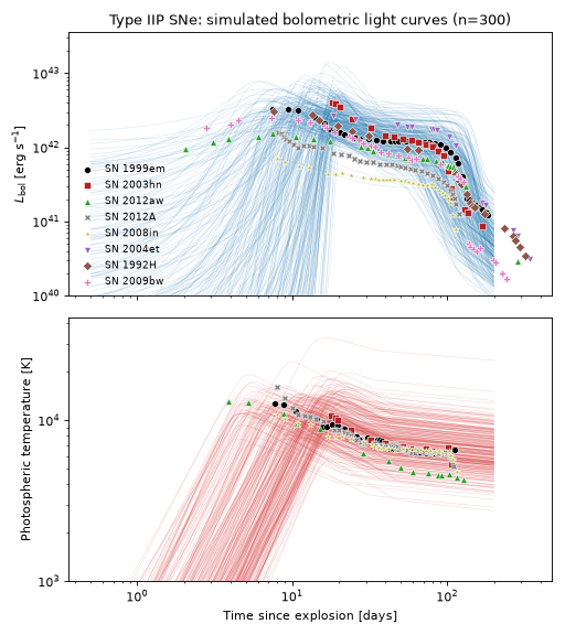
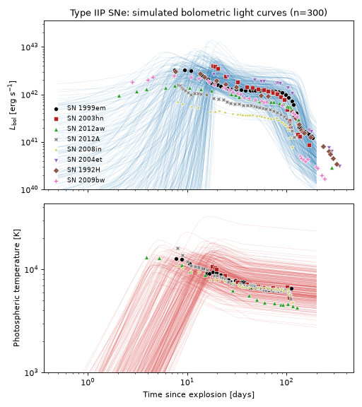
The plot below draws 300 random parameter realizations from the priors above and shows the resulting bolometric light curves and photospheric temperatures, overlaid with the observed light curves and temperatures of several Type IIP SNe [5][6].

(Source code, png, hires.png, pdf)

Observability Summary

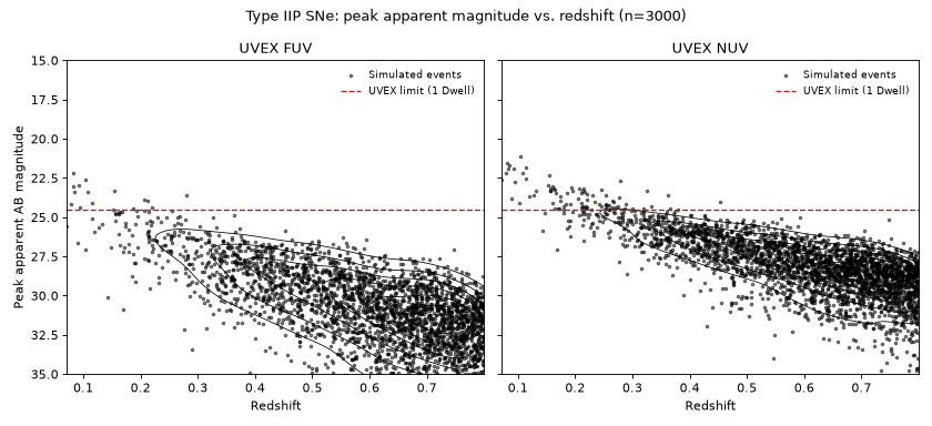
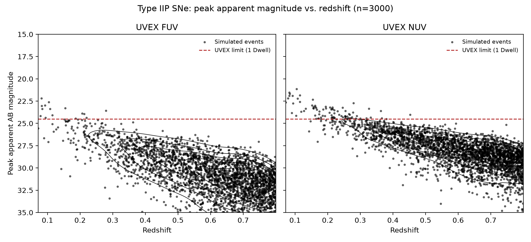
Below are the redshifts \(z\) and corresponding bandpass calculated peak apparent AB magnitudes \(m_\mathrm{AB}\) of 3000 simulated events drawn from the priors above, with the UVEX 1 Dwell limit of \(m<24.5\) overplotted. Because the bolometric light curve does not peak exactly at a single named parameter, the peak apparent magnitude is found by a numerical search over each event’s light curve rather than evaluated at a fixed time.

(Source code, png, hires.png, pdf)

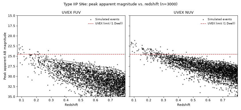
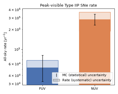
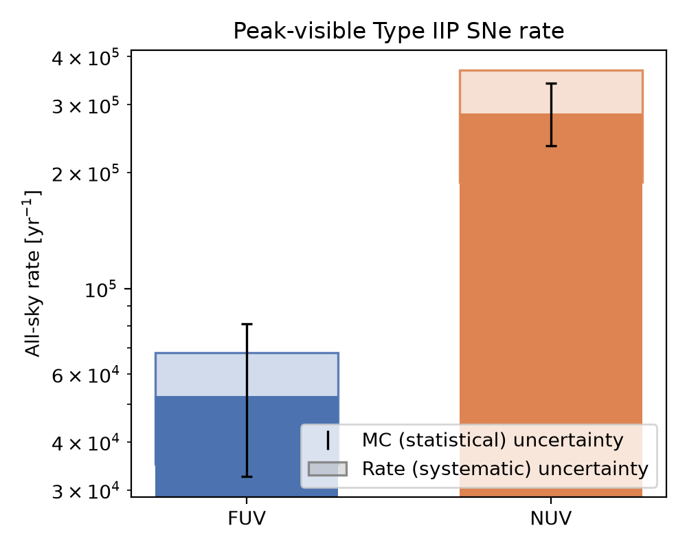
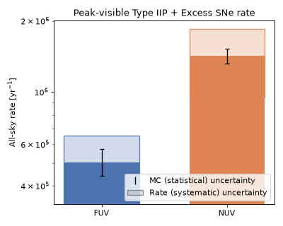
The anticipated rate detectable by UVEX at these limits is as follows, assuming that any event above the \(m<24.5\) limit is detectable, and that the population is isotropic and homogeneous in comoving volume out to its redshift limit:

(Source code, png, hires.png, pdf)

Type IIP + Excess

Implemented by TypeIIPExcessSNe, pairing TypeIIPExcessSED with the rate/duration metadata described below. IXF/GGI-like: a bright, hot, fast early excess on top of the same ordinary Type IIP evolution, attributed to shock breakout through and/or collisional heating of close circumstellar material.

Quick Facts

Quantity	Value	Source	Notes
Rate	30% of the Type IIP rate (14.6% of \(R_\mathrm{CC}(z)\))	Bruch et al.[7]	Reflects the high incidence of early CSM-interaction signatures found among Type II SNe (ZTF). The 30% multiplier has no published uncertainty of its own, so RATE_CI carries exactly the same relative uncertainty as ordinary Type IIP’s.
Redshift limit	\(z = 2\)	–	Higher than ordinary Type IIP, to admit this population’s brighter, more UV-luminous early-cooling realizations.
Duration	100 days	–	Same window as ordinary Type IIP.

SED Model

TypeIIPExcessSED is a subclass of TypeIIPSED: the same light curve and temperature functional forms,

\[L_\mathrm{bol}(t) = S_0(t)\,\bigl[1-S_P(t)\bigr] \Bigl[L_\mathrm{pk}\,e^{-(t-t_0)/\tau_\mathrm{cool}} + L_p\Bigr] + S_P(t)\, L_\mathrm{Co}\, e^{-(t-t_P)/\tau_\mathrm{Co}}, \qquad T(t) = T_0\, \left(\frac{t}{t_0}\right)^{\alpha_r} \left(\frac{1 + (t/t_0)^{s_0}}{2}\right)^{\frac{\alpha_c - \alpha_r}{s_0}} \left(\frac{1 + (t/\sqrt{t_0 t_P})^{s_1}}{2}\right)^{-\frac{\alpha_c - \alpha_p}{s_1}},\]

only with different parameter priors – an earlier, faster rise (t0, tau_rise), a higher peak luminosity (L_pk) and normalization temperature (T_0), and a shallower early-regime temperature index (alpha_r) – shifted to match the brighter, hotter, faster early cooling phase seen in SN 2023ixf and SN 2024ggi, rather than the smoother early decline of ordinary Type IIP SNe.

Parameter priors

Hand-tuned against SN 2023ixf [8] and SN 2024ggi [9], the only two objects of this kind currently in test_data/transients. Parameters not listed below (tau_drop, tau_Co) are fixed to the same values as ordinary Type IIP.

Parameter	Symbol	Prior	Notes
t0	\(t_0\)	Uniform(2 d, 5 d)	Explosion/rise reference epoch.
tau_rise	\(\tau_\mathrm{rise}\)	Normal(\(\log_{10}(\tau_\mathrm{rise}/\mathrm{d})\); mean=-0.5, \(\sigma\)=0.2)	Rise timescale (median \(\sim0.3\) d).
L_pk	\(L_\mathrm{pk}\)	Normal(\(\log_{10}(L_\mathrm{pk}/\mathrm{erg\,s^{-1}})\); mean=43.3, \(\sigma\)=0.25)	Early cooling-phase peak luminosity scale (median \(\sim2\times10^{43}\) erg/s).
tau_cool	\(\tau_\mathrm{cool}\)	Uniform(4 d, 15 d)	Early cooling-phase decay timescale.
L_p	\(L_p\)	Normal(\(\log_{10}(L_p/\mathrm{erg\,s^{-1}})\); mean=42.2, \(\sigma\)=0.2)	Plateau luminosity.
t_P	\(t_P\)	Uniform(50 d, 150 d)	Plateau-end / radioactive-tail-onset epoch.
L_Co	\(L_\mathrm{Co}\)	Normal(\(\log_{10}(L_\mathrm{Co}/\mathrm{erg\,s^{-1}})\); mean=41.5, \(\sigma\)=0.3)	Radioactive-tail luminosity at t_P.
T_0	\(T_0\)	Normal(\(\log_{10}(T_0/\mathrm{K})\); mean=4.2, \(\sigma\)=0.1)	Normalization: \(T(t_0) \approx T_0\) (\(\sim1.6\times10^4\) K).
alpha_r	\(\alpha_r\)	Normal(1, \(\sigma\)=0.2)	Early-regime power-law index; \(T\) rises toward \(t_0\).
alpha_c	\(\alpha_c\)	Normal(-0.45, \(\sigma\)=0.1)	Cooling-regime power-law index; \(T\) declines.
alpha_p	\(\alpha_p\)	Normal(-0.1, \(\sigma\)=0.01)	Plateau-regime power-law index; \(T\) declines slowly.
s_0	\(s_0\)	Uniform(10, 20)	Sharpness of the break at \(t_0\).
s_1	\(s_1\)	Uniform(10, 50)	Sharpness of the break at \(\sqrt{t_0 t_P}\).

Simulated Light Curves

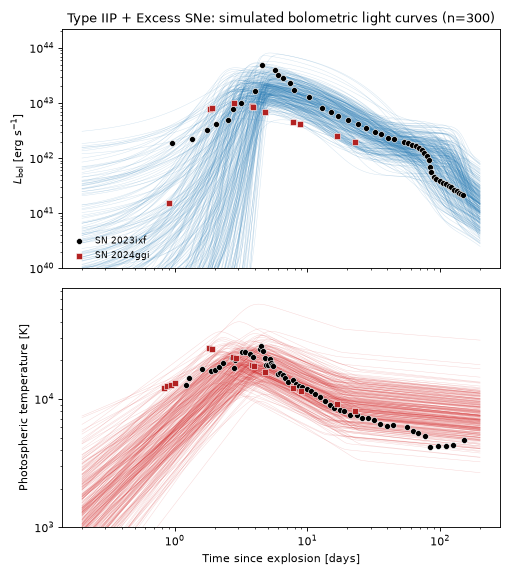
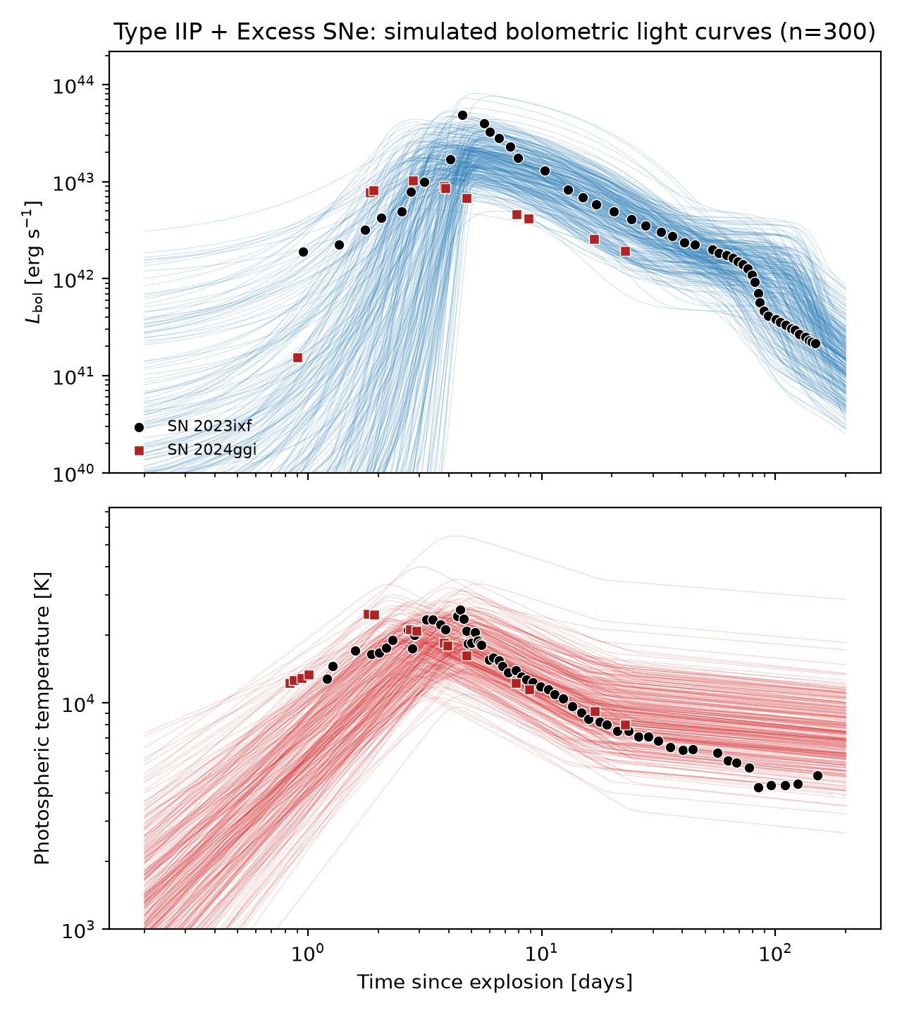
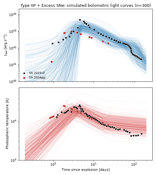
The plot below draws 300 random parameter realizations from the priors above and shows the resulting bolometric light curves and photospheric temperatures, overlaid with the observed light curves and temperatures of SN 2023ixf [8] and SN 2024ggi [9].

(Source code, png, hires.png, pdf)

Observability Summary

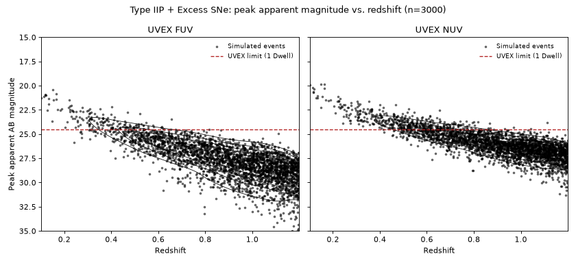
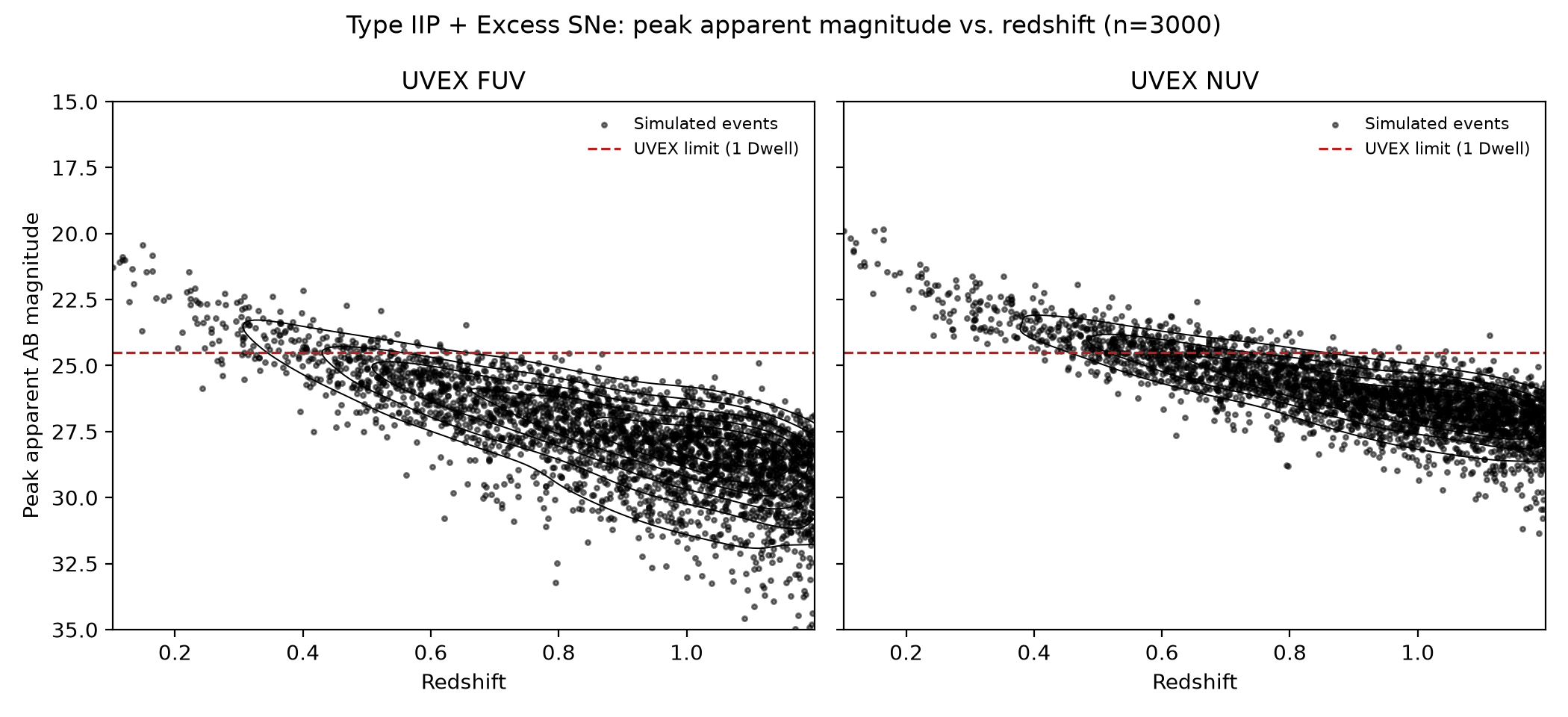
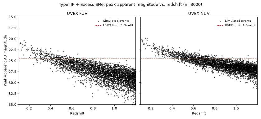
Below are the redshifts \(z\) and corresponding bandpass calculated peak apparent AB magnitudes \(m_\mathrm{AB}\) of 3000 simulated events drawn from the priors above, with the UVEX 1 Dwell limit of \(m<24.5\) overplotted.

(Source code, png, hires.png, pdf)

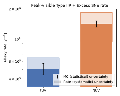
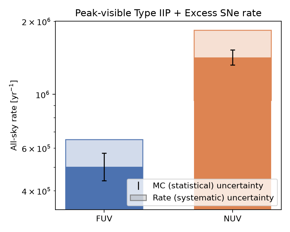
The anticipated rate detectable by UVEX at these limits is as follows, assuming that any event above the \(m<24.5\) limit is detectable, and that the population is isotropic and homogeneous in comoving volume out to its redshift limit:

(Source code, png, hires.png, pdf)

Type IIb

Type IIb supernovae are core-collapse explosions of massive stars that have been stripped of most, but not all, of their hydrogen envelope. Many show a double-peaked light curve: an early, hours- to-days-long flash powered by the shock heating and subsequent cooling of the extended envelope, followed – after a dip – by a broader, weeks-long peak powered by radioactive \(^{56}\mathrm{Ni}\) decay, the same mechanism that powers most other core-collapse SN light curves. Others show only the single, radioactively powered peak, with no resolved early bump. Where ShockCoolingIIb models only the shock-cooling component from first principles, this population is a purely phenomenological light curve intended to span the whole population – single- and double-peaked events alike – in a single functional form.

This population is implemented by TypeIIbSNe, pairing TypeIIbSED with the rate/duration metadata described below.

Note

The priors below are broad, order-of-magnitude-motivated ranges, not yet a fit to any specific real Type IIb event. This page will be updated if/when they are recalibrated against data (as TypeIIPSED was).

Quick Facts

Quantity	Value	Source	Notes
Rate	\(R_\mathrm{CC}(z) = k\,\psi_\mathrm{UV}(z)\); Type IIb 10.3% of \(R_\mathrm{CC}(z)\)	Strolger et al.[1], Madau and Dickinson[2], Shivvers et al.[4]	Tracks the cosmic star-formation history. Shivvers et al.[4] find IIb is \(34.0\pm11.1\%\) of the stripped-envelope (SESNe) rate, which is itself \(30.4^{+5.0}_{-4.9}\%\) of the total core-collapse rate, so the Type IIb fraction of the CC rate is \(0.340\times0.304=0.103\). Combined in quadrature with Strolger et al.[1]’s \(+27\%/-31\%\) normalization uncertainty, this gives RATE_CI (see Rate Uncertainty and All-Sky Yield). Identical rate to ShockCoolingIIb – both describe the same underlying Type IIb population, just with different SED models.
Redshift limit	\(z = 0.5\)	–	Tighter than the \(z = 1\) bound of ShockCoolingIIb.
Duration	200 days	–	Long enough to cover the shock-cooling peak (where present), the dip, the radioactive main peak, and its subsequent decline – unlike ShockCoolingIIb’s much shorter 20 day window, which covers only the first of those phases.

SED Model

TypeIIbSED pairs a superposition of two Bazin pulses with the same single-power-law cooling blackbody photosphere used elsewhere in this package (e.g. VillarCoolingBlackbodySED):

\[L_\mathrm{bol}(t) = A_0\, \frac{\exp[-(t-t_0)/\tau_{\mathrm{fall},0}]}{1 + \exp[-(t-t_0)/\tau_{\mathrm{rise},0}]} + A_1\, \frac{\exp[-(t-t_1)/\tau_{\mathrm{fall},1}]}{1 + \exp[-(t-t_1)/\tau_{\mathrm{rise},1}]}, \qquad T(t) = T_\mathrm{floor} + (T_0 - T_\mathrm{floor})\left(1 + \frac{t}{\tau_T}\right)^{-\alpha_T}.\]

The light curve is delegated directly to TwoComponentBazinLightcurve: two ordinary BazinLightcurve pulses, added rather than multiplied – an early one centered on \(t_0\) standing in for the shock-cooling peak, and a later one centered on \(t_1\) for the radioactively powered main peak. Because the two components are independent and additive, a single functional form covers both populations at once: with the early component’s amplitude \(A_0\) much smaller than the main peak’s \(A_1\), only the main peak is visible (a single-peaked event); with \(A_0\) comparable to \(A_1\), both peaks show, with a dip between them where each pulse has decayed enough for the other to dominate (a double-peaked event). This fits real double- and single-peaked Type IIb light curves better than a single pulse reshaped by a multiplicative modulation.

Parameter priors

amplitude_0 – the early peak’s normalization – is uniform in \(\log_{10}(A_0/\mathrm{erg\,s^{-1}})\) between 39 and 43, i.e. from \(10^{39}\) to \(10^{43}\ \mathrm{erg\,s^{-1}}\): far fainter than the main peak (an effectively single-peaked draw) up to brighter than it (a double-peaked, or even early-peak-dominated, draw); roughly a third of draws from the priors below are double-peaked. t0 and T_floor are held fixed; every other parameter is drawn from a broad Uniform (or, for amplitude_1/T0, Normal-in-log) prior.

Parameter	Symbol	Prior	Notes
amplitude_0	\(A_0\)	LogUniform(\(10^{39}\), \(10^{43}\ \mathrm{erg\,s^{-1}}\))	Early, shock-cooling peak normalization; spans negligible to brighter than the main peak.
t0	\(t_0\)	Fixed (2 d)	Transition time of the early peak.
rise_0	\(\tau_{\mathrm{rise},0}\)	Uniform(0.3 d, 1 d)	Logistic rise timescale of the early peak.
fall_0	\(\tau_{\mathrm{fall},0}\)	Uniform(3 d, 10 d)	Exponential decline timescale of the early peak.
amplitude_1	\(A_1\)	Normal(\(\log_{10}(A_1/\mathrm{erg\,s^{-1}})\); mean=42.5, \(\sigma\)=0.1)	Main, radioactively powered peak normalization (median \(\sim3\times10^{42}\) erg/s).
t1	\(t_1\)	Uniform(10 d, 20 d)	Transition time of the main peak.
rise_1	\(\tau_{\mathrm{rise},1}\)	Uniform(2 d, 4 d)	Logistic rise timescale of the main peak.
fall_1	\(\tau_{\mathrm{fall},1}\)	Uniform(30 d, 55 d)	Exponential decline timescale of the main peak.
T0	\(T_0\)	Normal(\(\log_{10}(T_0/\mathrm{K})\); mean=4.1, \(\sigma\)=0.05)	Photospheric temperature as \(t \to 0\) (median \(\sim1.3\times10^4\) K).
T_floor	\(T_\mathrm{floor}\)	Fixed (\(4\times10^3\) K)	Asymptotic late-time photospheric temperature.
tau_T	\(\tau_T\)	Uniform(5 d, 10 d)	Photospheric cooling timescale.
alpha_T	\(\alpha_T\)	Uniform(0.7, 1.3)	Photospheric cooling power-law index.

Simulated Light Curves

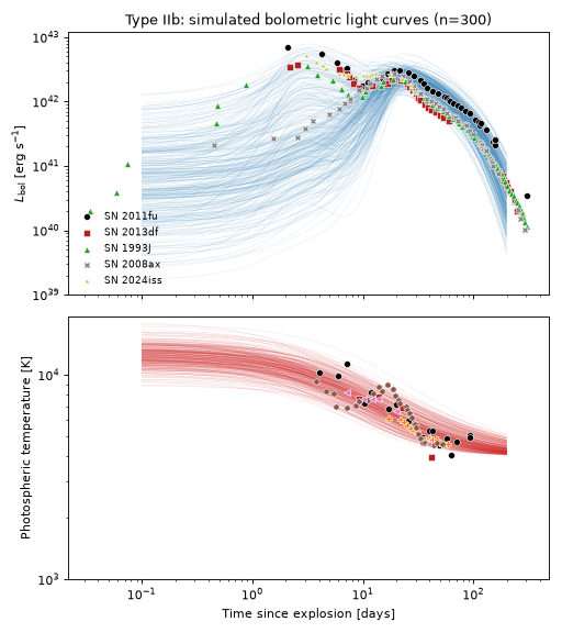
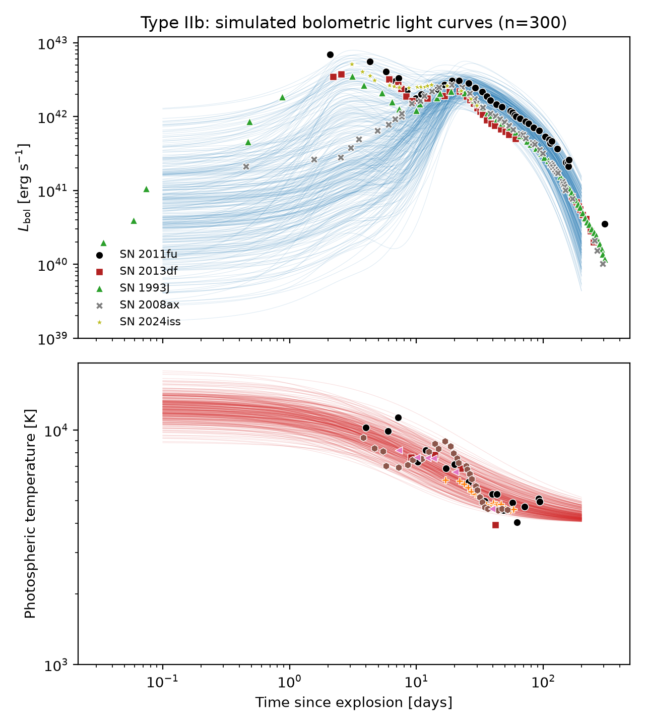
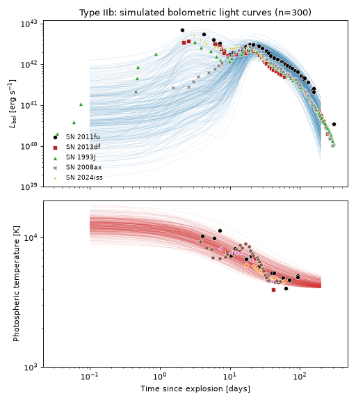
The plot below draws 300 random parameter realizations from the priors above and shows the resulting bolometric light curves and photospheric temperatures, overlaid with the observed light curves and temperatures of several Type IIb SNe [10][11][12][13][14][15]. The spread illustrates the single-/double-peaked split described above: most realizations show only the main peak, with a minority showing a distinct early bump or, at the high end of the amplitude_0 prior, an early-dominated light curve – both SN 1993J and SN 2011fu are well-known double-peaked events, and show up as such in the overlaid data.

(Source code, png, hires.png, pdf)

Observability Summary

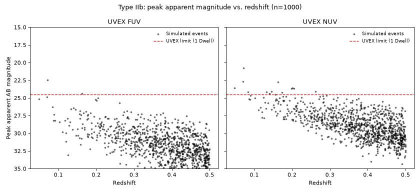
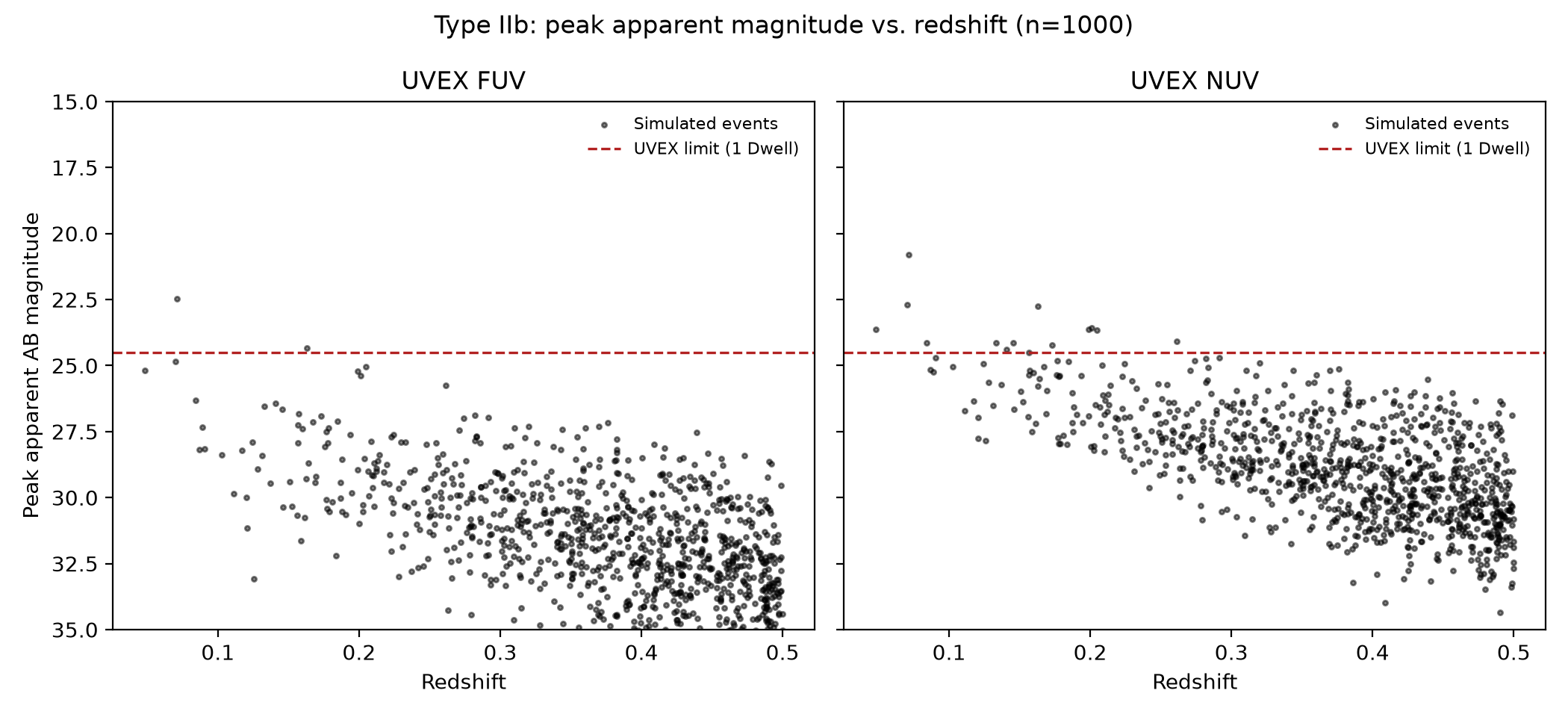
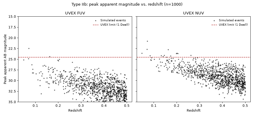
Below are the redshifts \(z\) and corresponding bandpass peak apparent AB magnitudes \(m_\mathrm{AB}\) of 1000 simulated events drawn from the priors above, with the UVEX 1 Dwell limit of \(m<24.5\) overplotted. The peak apparent magnitude is found by a numerical search over each event’s light curve, since neither peak sits at a single named parameter once both components contribute.

(Source code, png, hires.png, pdf)

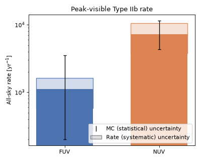
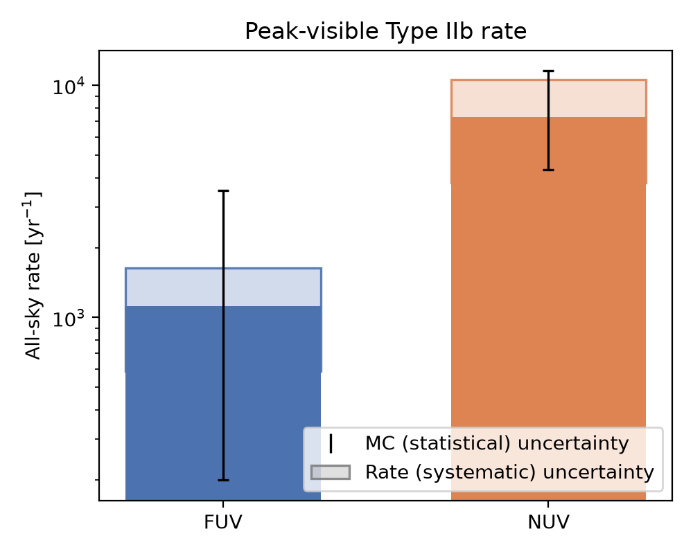
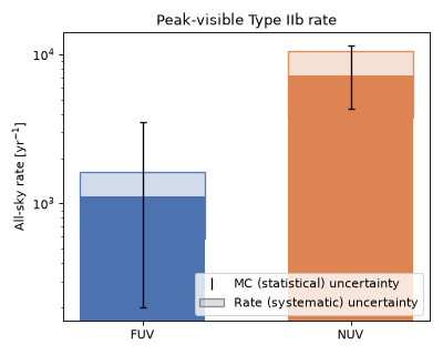
The anticipated rate detectable by UVEX at this limit is as follows, assuming that any event above the \(m<24.5\) limit is detectable, and that the population is isotropic and homogeneous in comoving volume out to its redshift limit:

(Source code, png, hires.png, pdf)

References

[1] (1,2,3,4)

Louis-Gregory Strolger, Tomas Dahlen, Steven A. Rodney, Or Graur, Adam G. Riess, Curtis McCully, Swara Ravindranath, Bahram Mobasher, and A. Kristin Shahady. The rate of core collapse supernovae to redshift 2.5 from the CANDELS and CLASH supernova surveys. The Astrophysical Journal, 813(2):93, 2015. arXiv:1509.06574, doi:10.1088/0004-637X/813/2/93.

[2] (1,2)

Piero Madau and Mark Dickinson. Cosmic star-formation history. Annual Review of Astronomy and Astrophysics, 52:415–486, 2014. arXiv:1403.0007, doi:10.1146/annurev-astro-081811-125615.

[3] (1,2)

Weidong Li, Jesse Leaman, Ryan Chornock, Alexei V. Filippenko, Dovi Poznanski, Mohan Ganeshalingam, Xiaofeng Wang, Maryam Modjaz, Saurabh Jha, Ryan J. Foley, and Nathan Smith. Nearby supernova rates from the lick observatory supernova search. ii. the observed luminosity functions and fractions of supernovae in a complete sample. Monthly Notices of the Royal Astronomical Society, 412(3):1441, 2011. arXiv:1006.4612, doi:10.1111/j.1365-2966.2011.18160.x.

[4] (1,2,3,4)

Isaac Shivvers, Maryam Modjaz, WeiKang Zheng, Yuqian Liu, Alexei V. Filippenko, Jeffrey M. Silverman, Thomas Matheson, Andrea Pastorello, Or Graur, Ryan J. Foley, Ryan Chornock, Nathan Smith, Jesse Leaman, and Stefano Benetti. Revisiting the lick observatory supernova search volume-limited sample: updated classifications and revised stripped-envelope supernova fractions. Publications of the Astronomical Society of the Pacific, 129(975):054201, 2017. arXiv:1609.02922, doi:10.1088/1538-3873/aa54a6.

[5]

M. Dall’Ora, M. T. Botticella, M. L. Pumo, L. Zampieri, L. Tomasella, G. Pignata, and others. The type IIP supernova 2012aw in M95: hydrodynamical modelling of the photospheric phase from accurate spectrophotometric monitoring. The Astrophysical Journal, 787:139, 2014. arXiv:1404.1294, doi:10.1088/0004-637X/787/2/139.

[6]

Tamar Faran, Ehud Nakar, and Dovi Poznanski. The evolution of temperature and bolometric luminosity in type-II supernovae. Monthly Notices of the Royal Astronomical Society, 473:513–537, 2018. arXiv:1707.07695, doi:10.1093/mnras/stx2288.

[7]

Rachel J. Bruch, Avishay Gal-Yam, Offer Yaron, Ping Chen, Nora L. Strotjohann, Ido Irani, Erez Zimmerman, and others. The prevalence and influence of circumstellar material around hydrogen-rich supernova progenitors. The Astrophysical Journal, 952:119, 2023. arXiv:2212.03313, doi:10.3847/1538-4357/acd8be.

[8] (1,2)

Brian Hsu, Nathan Smith, Jared A. Goldberg, K. Azalee Bostroem, Griffin Hosseinzadeh, David J. Sand, Jeniveve Pearson, Daichi Hiramatsu, Jennifer E. Andrews, and Emma R. Beasor. One year of SN 2023ixf: breaking through the degenerate parameter space in light-curve models with pulsating progenitors. The Astrophysical Journal, 2025. arXiv:2408.07874, doi:10.3847/1538-4357/adf222.

[9] (1,2)

Xinlei Chen, Brajesh Kumar, Xinzhong Er, Helong Guo, Yuan-Pei Yang, Weikang Lin, Yuan Fang, Guowang Du, Chenxu Liu, and Jiewei Zhao. Early-phase simultaneous multiband observations of the type ii supernova SN 2024ggi with mephisto. The Astrophysical Journal Letters, 971:L2, 2024. arXiv:2405.07964.

[10]

Michael W. Richmond, Richard R. Treffers, Alexei V. Filippenko, Yong Paik, Bruno Leibundgut, Eric Schulman, and Colin V. Cox. UBVRI photometry of the type II supernova 1993j in M81: the first 120 days. The Astronomical Journal, 107:1022, 1994. doi:10.1086/116915.

[11]

S. Taubenberger, H. Navasardyan, J. I. Maurer, L. Zampieri, E. Kankare, A. Pastorello, and others. High-precision multicolour light curves of the type IIb SN 2008ax and its early flux excess. Monthly Notices of the Royal Astronomical Society, 413:2140–2154, 2011. arXiv:1101.5171, doi:10.1111/j.1365-2966.2011.18287.x.

[12]

A. Morales-Garoffolo, N. Elias-Rosa, M. Bersten, E. Baron, S. Benetti, and others. The type IIb supernova 2013df: a close sibling of SN 1993j. Monthly Notices of the Royal Astronomical Society, 445:1647–1666, 2014. arXiv:1408.6242, doi:10.1093/mnras/stu1837.

[13]

A. Morales-Garoffolo, N. Elias-Rosa, S. Benetti, E. Cappellaro, S. D. Van Dyk, and others. SN 2011fu: half a million years in the life of a self-obscured type IIb supernova progenitor. Monthly Notices of the Royal Astronomical Society, 454:95–116, 2015. arXiv:1508.05427, doi:10.1093/mnras/stv1972.

[14]

Masayuki Yamanaka, Takahiro Nagayama, and Tsukiha Horikiri. SN 2024iss: double-peaked light curves and implications for a yellow supergiant progenitor. Publications of the Astronomical Society of Japan, 2025. accepted. arXiv:2503.05054.

[15]

S. J. Prentice, C. Ashall, P. A. James, L. Short, P. A. Mazzali, D. Bersier, P. A. Crowther, C. Barbarino, T.-W. Chen, C. M. Copperwheat, M. J. Darnley, L. Denneau, N. Elias-Rosa, M. Fraser, L. Galbany, A. Gal-Yam, J. Harmanen, D. A. Howell, G. Hosseinzadeh, C. Inserra, E. Kankare, E. Karamehmetoglu, G. P. Lamb, M. Limongi, K. Maguire, C. McCully, F. Olivares E., A. S. Piascik, G. Pignata, D. E. Reichart, A. Rest, T. Reynolds, Ó. Rodríguez, J. L. O. Saario, S. Schulze, S. J. Smartt, K. W. Smith, J. Sollerman, B. Stalder, M. Sullivan, F. Taddia, S. Valenti, S. D. Vergani, S. C. Williams, and D. R. Young. Investigating the properties of stripped-envelope supernovae; what are the implications for their progenitors? Monthly Notices of the Royal Astronomical Society, 485(2):1559–1578, 2019. arXiv:1812.03716, doi:10.1093/mnras/sty3399.