Transients#

uvex_transients.transients sits between the SED framework in uvex_transients.models and the survey pipeline in uvex_transients.simulation. A TransientBase subclass is a thin pairing of one SpectralModel (sed) with the metadata needed to window a survey simulation around it – above all, a strict upper bound on how long the transient could plausibly stay relevant (duration_limit). Its ExtragalacticTransient subclass adds a cosmological volumetric event rate, turning that pairing into something that can draw its own Monte Carlo population: given a comoving rate density and a patch of sky and time, how many events exploded there, at what redshifts, and when.

This page covers that shared machinery – TransientBase/ExtragalacticTransient themselves, not any one population. For the astrophysics, adopted rate, SED choice, and default parameter priors of each implemented population (kilonovae, TDEs, LFBOTs, supernovae), see the Transients gallery instead; for how SurveySimulator drives this sampling against a real survey schedule, see Simulation.

Quick Look#

Every transient class is instantiated with no arguments – everything below works identically for any of the built-in populations, so this page uses TidalDisruptionEvent throughout as a running example:

import numpy as np
import matplotlib.pyplot as plt
from astropy import units as u

from uvex_transients.transients.TDEs import TidalDisruptionEvent

tde = TidalDisruptionEvent()

print(tde.sed)                  # the VanVelzenTDESED SED instance
print(tde.duration_limit)       # 200.0 d
print(tde.redshift_limit)       # 2

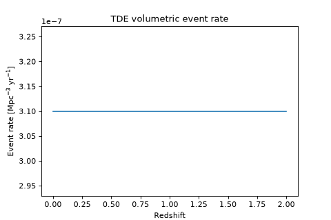
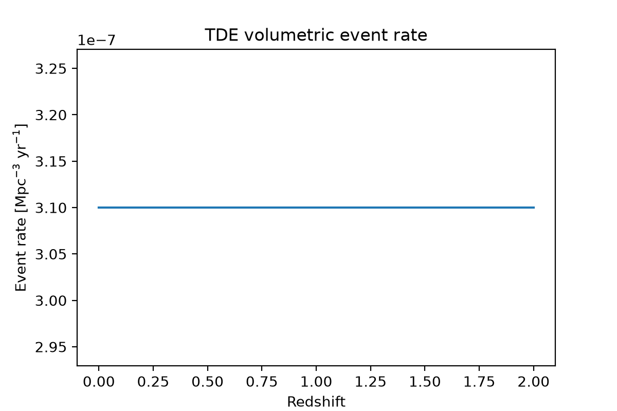
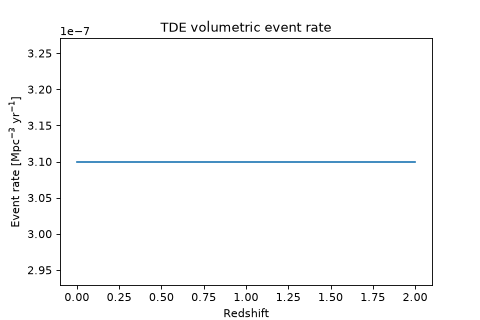
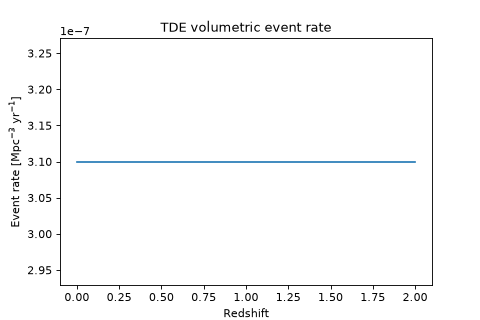
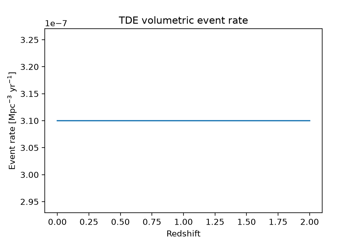
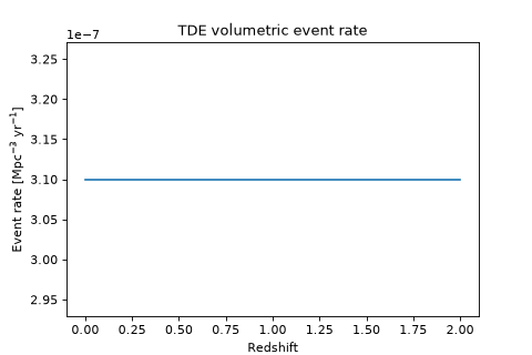
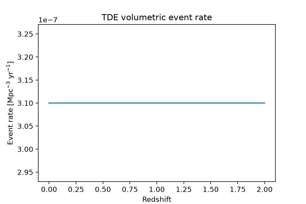
z = np.linspace(0, tde.redshift_limit, 200)
rate = tde.event_rate(z)

fig, ax = plt.subplots(figsize=(6, 4))
ax.plot(z, rate)
ax.set_xlabel("Redshift")
ax.set_ylabel(r"Event rate [Mpc$^{-3}$ yr$^{-1}$]")
ax.set_title("TDE volumetric event rate")

(Source code, png, hires.png, pdf)

A transient class is a pairing: sed is exactly the SpectralModel documented in Models (every eval/flux/mag method, every prior, sample_parameters, all of it), and duration_limit/event_rate are the two pieces of extra bookkeeping that let ExtragalacticTransient turn that SED into a self-sampling population, covered below.

The Transient Object#

TransientBase itself is deliberately minimal: it holds one SED instance and one duration, and nothing about how many events exist or where – that’s ExtragalacticTransient’s job, covered in the next two sections.

tde.sed              # the VanVelzenTDESED instance -- see user_guide_models
tde.duration_limit    # 200.0 d
tde.cosmology         # the astropy Cosmology used for D_L(z) and comoving volume

tde.duration_limit = 90 * u.day   # override -- must be a positive time Quantity

A concrete subclass supplies exactly two class variables, checked at class-definition time (not buried inside __init__, so a subclass that forgets one fails immediately at import, not partway through a Monte Carlo run):

Class variable	Meaning
`DEFAULT_MODEL`	The `SpectralModel` subclass this transient type is built from; instantiated fresh (with its own default parameters/priors) for every new transient instance.
`DEFAULT_DURATION`	The default `duration_limit`: a strict upper bound on the time between explosion and the transient fading below any relevance, not a typical or characteristic duration – used for windowing, so an overly generous value costs some wasted sampling but an overly tight one silently drops real detections.

Twelve populations ship with the package today, each pairing one of these SEDs with a rate and duration – see the linked Transients page for each one’s astrophysics and priors:

Class	Default SED	Duration	Redshift limit
`Kilonova`	`KilonovaCoolingBlackbodySED`	30 d	0.2
`TidalDisruptionEvent`	`VanVelzenTDESED`	200 d	2
`LuminousFastBlueOpticalTransient`	`LFBOTCoolingBlackbodySED`	100 d	3
`TypeIIPSNe`	`TypeIIPSED`	100 d	0.8
`TypeIIPExcessSNe`	`TypeIIPExcessSED`	100 d	1.2
`TypeIIbSNe`	`TypeIIbSED`	200 d	0.5
`ShockCoolingIIb`	`MoragShockCoolingSED`	20 d	1
`TypeIbSNe`	`TypeIbSED`	100 d	0.5
`TypeIcSNe`	`TypeIcSED`	100 d	0.5
`TypeIcBLSNe`	`TypeIcBLSED`	100 d	0.5
`MagnetarSLSNe`	`ArnettMagnetarSpindownSED`	600 d	4
`TypeIaSNe`	`TypeIaSED`	365 d	1

Volumetric Rates and Redshift Sampling#

ExtragalacticTransient is the abstract base every extragalactic population above subclasses. Concrete subclasses implement two abstract members – rate, the fiducial rate normalization \(R_0\) (a single, possibly cosmology-dependent Quantity), and rate_shape(), the dimensionless redshift shape \(f(z)\) – rather than event_rate() directly. event_rate() itself is a thin, already-implemented product of the two, \(R(z;A)=A f(z)\), the comoving event rate density in events / Mpc³ / yr as a function of redshift. rate_shape must be NumPy-vectorized – called once, across a whole grid, never in a per-event loop:

tde.event_rate(0.5)                      # a scalar rate at z=0.5
tde.event_rate(np.linspace(0, 2, 50))    # the same function, vectorized

From Rate to a Redshift Distribution#

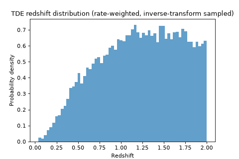
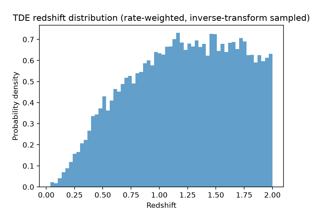
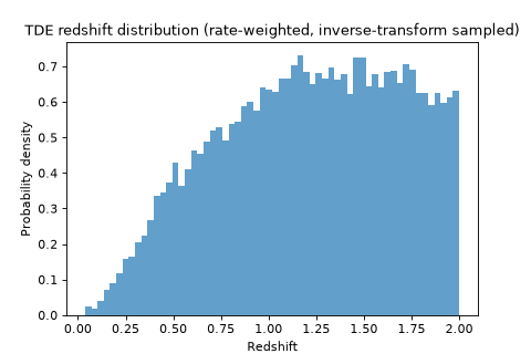
event_rate alone isn’t yet something you can sample from – it’s a rate density, not a probability distribution, and it needs to be weighted by the comoving volume element and the cosmological time-dilation between rest-frame rate and observer-frame duration. On first access, redshift_grid, luminosity_distance_grid, and integrated_rate all trigger one lazy build: event_rate is tabulated once, on a grid of redshift_grid_size points spanning [0, redshift_limit], weighted by

\[w(z) = R(z) \, \frac{dV_c}{dz} \Big/ (1+z),\]

then integrated (via cumulative trapezoidal quadrature) into both a total – integrated_rate, the expected count per steradian per unit observer time – and a CDF used to draw redshifts by inverse-transform sampling:

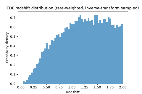
z_samples = tde.sample_event_redshift(20000, rng=0)

fig, ax = plt.subplots(figsize=(6, 4))
ax.hist(z_samples, bins=60, density=True, color="C0", alpha=0.7)
ax.set_xlabel("Redshift")
ax.set_ylabel("Probability density")
ax.set_title("TDE redshift distribution (rate-weighted, inverse-transform sampled)")

(Source code)

../../_images/overview-2_00.png — (`png`, `hires.png`, `pdf`)#

../../_images/overview-2_01.png — (`png`, `hires.png`, `pdf`)#

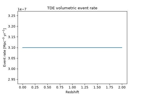
sample_event_redshift() is the one-line version of that inversion; luminosity_distance_grid caches \(D_L(z)\) at the same grid points, so a caller with a batch of already-sampled redshifts gets \(D_L\) via a cheap numpy.interp() against it rather than a second cosmology.luminosity_distance call (exactly what generate_events() does – see Simulation).

Important

All of this is cached and rebuilt lazily, keyed off (cosmology, redshift_limit, redshift_grid_size) – reassigning any of cosmology, redshift_limit, or redshift_grid_size invalidates the cache, so the next access rebuilds it against the new value rather than silently reusing a stale one. event_rate itself is only ever evaluated once per rebuild, no matter how many events are subsequently sampled from it.

Rate Uncertainty and All-Sky Yield#

Everything above assumes the rate normalization \(R_0=\) rate is known exactly. In practice, a literature rate comes with its own uncertainty, and Yield Statistics derives confidence bounds throughout that carry it through to a final expected-detection estimate. On the transient class itself, that uncertainty is a single class variable:

TidalDisruptionEvent.RATE_CI              # (0.6774..., 1.1935...) -- multiplicative (lower, upper) factors
Kilonova.RATE_CI                          # (0.2545..., 2.7454...) -- multiplicative (lower, upper) factors
LuminousFastBlueOpticalTransient.RATE_CI  # (0.09, 1.25) -- multiplicative (lower, upper) factors
TypeIaSNe.RATE_CI                         # (0.9231, 1.0769) -- multiplicative (lower, upper) factors

RATE_CI is a pair of multiplicative factors on rate (not absolute bounds), at a 90% confidence level by convention – if a publication reports \(R_0{}^{+\Delta R_+}_{-\Delta R_-}\), that’s ((R_0 - dR_minus) / R_0, (R_0 + dR_plus) / R_0). Multiplicative factors, rather than a fixed Quantity pair, mean the same RATE_CI applies unchanged to a rate that is itself cosmology-dependent. Every built-in population currently has a RATE_CI sourced from the literature (see the Transients gallery for each one’s derivation), but None remains its default on ExtragalacticTransient itself – the starting point for any new custom subclass, and what a class falls back to if it’s ever ahead of the literature. Leaving it at that default means no rate uncertainty has been sourced yet – every bound below then collapses to the point estimate, twice over, rather than silently reading as “the rate is known exactly.”

Every rate-derived quantity has a plain point-estimate property and a ..._ci-suffixed bounds counterpart built from RATE_CI:

Point estimate	Bounds	Meaning
`rate`	`rate_ci`	The fiducial normalization \(R_0\) itself.
`integrated_rate`	`integrated_rate_ci`	Per-steradian, per-observer-year rate integrated over redshift (see above).
`all_sky_rate`	`all_sky_rate_ci`	`integrated_rate` restored to the full \(4\pi\) sky.
`compute_all_sky_yield()`	`compute_all_sky_yield_ci()`	`all_sky_rate` times an observer-frame duration – the expected intrinsic event count over the whole sky and that window, with no survey footprint or detection selection applied.

None of these know anything about a particular survey’s footprint – they’re the \(\mu_0\) that ExposureCatalog and compute_yield_summary() restrict down to the footprint an actual schedule swept out (see Simulation). effective_volume (\(\mathcal V\) in Yield Statistics) is the rate-weighted comoving volume integrated_rate is built from, with rate’s own normalization divided back out – it depends only on rate_shape, cosmology, and redshift_limit, so it carries no rate-normalization uncertainty of its own.

See Yield Statistics for the full derivation of every bound above, and Simulation for how they combine with a real survey schedule’s footprint and a Monte Carlo catalog’s detection efficiency into a final yield estimate.

Sampling Events#

With a redshift distribution in hand, ExtragalacticTransient can draw an actual Monte Carlo population: how many events, where, when, and with which SED parameters.

How Many Events#

sample_event_count() converts integrated_rate into an expected count over a given solid angle and duration, then draws a Poisson realization of it:

n = tde.sample_event_count(solid_angle=100 * u.deg**2, duration=180 * u.day, seed=0)

duration above can also be given as a t_start/t_end pair instead – both sample_event_count and sample_events_on_healpix_grid below resolve it the same way.

Drawing a Full Population#

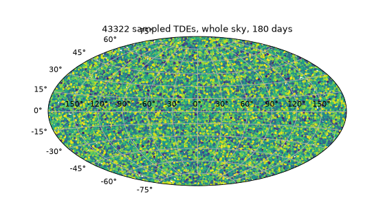
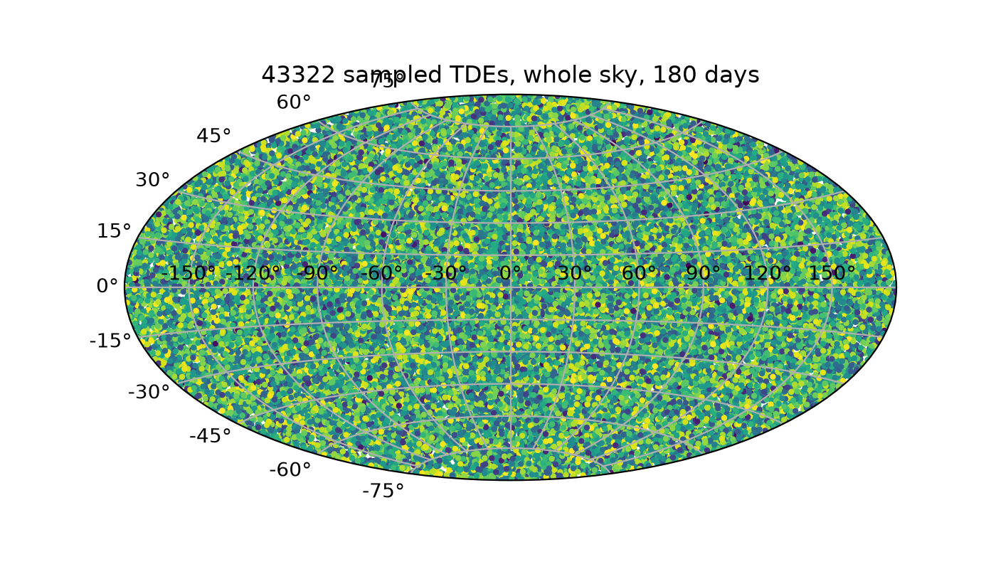
sample_events_on_healpix_grid() is the main event: it draws the count above, then places each event uniformly at random within one of a set of eligible HEALPix pixels (optionally jittered to a sub-pixel position via jitter; see below), assigns it a redshift from sample_event_redshift, an explosion time drawn uniformly across the sampling window, and a per-event parameter seed – rather than fully-sampled physical SED parameters, which are meant to be regenerated lazily, on demand, from that seed (see Parameter Seeds, Not Parameters below).

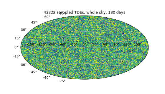
from astropy.time import Time

events = tde.sample_events_on_healpix_grid(
    nside=32,
    t_start=Time("2025-01-01"),
    duration=180 * u.day,
    seed=0,
)
print(f"Sampled {len(events)} events.")

fig = plt.figure(figsize=(7, 4))
ax = fig.add_subplot(111, projection="aitoff")
ax.grid(True)
ra = events["coord"].ra.wrap_at(180 * u.deg).radian
ax.scatter(ra, events["coord"].dec.radian, s=4, c=events["redshift"], cmap="viridis")
ax.set_title(f"{len(events)} sampled TDEs, whole sky, 180 days")

(Source code)

../../_images/overview-3_00.png — (`png`, `hires.png`, `pdf`)#

../../_images/overview-3_01.png — (`png`, `hires.png`, `pdf`)#

../../_images/overview-3_02.png — (`png`, `hires.png`, `pdf`)#

By default every pixel of the nside grid is eligible, as above; pixel_mask (a boolean mask over the full grid) or pixel_ids (an explicit array of pixel indices) restrict sampling to a subset – exactly how generate_events() restricts each time bin’s sampling to only the HEALPix pixels the survey schedule actually observed during that bin (see Simulation), rather than sampling the whole sky and discarding almost everything.

The returned table has one row per sampled event:

Column	Type	Meaning
`healpix_id`	int	Sampling pixel, at the `nside`/`order` passed in.
`healpix_dx`, `healpix_dy`	float	Sub-pixel offset within `healpix_id` (`0.5, 0.5` for every event if `jitter=False`).
`coord`	`SkyCoord`	Sky position, derived from `healpix_id`/`healpix_dx`/`healpix_dy`.
`redshift`	float	Drawn from `sample_event_redshift`.
`t_explosion`	`Time`	Drawn uniformly across `[t_start, t_start + duration)`.
`parameter_seed`	int	Regenerates this event’s physical SED parameters on demand – see below.

Parameter Seeds, Not Parameters#

Notice what’s not in that table: no amplitude, no rise time, no temperature – none of the SED’s own physical parameters. Sampling a full parameter set for every event up front would be wasted work for the overwhelming majority of a freshly-sampled population that never survives screening (see filter_by_limiting_magnitude() in Simulation), and would mean sample_events_on_healpix_grid’s own output schema depends on which SED a transient type happens to use. Instead, only a parameter_seed is stored – one independent, individually-storable seed per event (drawn from a single spawned tree, so no two events, however many are sampled, ever share a stream) – and the actual parameters are regenerated from it later, exactly once needed, via sample_parameters():

seed = int(events["parameter_seed"][0])
params = tde.sed.sample_parameters(size=1, rng=np.random.default_rng(seed))

This is exactly what sample_parameters() does for a single reconstructed event, and what filter_by_limiting_magnitude()/ filter_by_snr() do in batch across a whole catalog – see Simulation for both.

Reproducibility#

Every stochastic call on this page takes a seed/rng argument (an integer, an existing numpy.random.Generator, or None for non-reproducible entropy), the same way sample_parameters() does in Models. sample_events_on_healpix_grid in particular spawns one tree of independent child streams from its own seed – one per stochastic draw it makes internally (the event count, pixel assignment, jitter, explosion time, redshift, and the parameter-seed spawn point itself) – so that no two of those draws, and no two sampled events’ own parameter_seed values, can ever collide, regardless of how many events end up being sampled. The same seed therefore always reproduces the same population, down to the last parameter_seed.

See the Transients gallery for the astrophysics, adopted rate, and default priors of each implemented population, Writing a Custom Transient for writing your own, and uvex_transients.transients in the API reference for exhaustive method-by-method detail.