Shock-Cooling Emission from Type IIb SNe

Type IIb supernovae are core-collapse explosions of massive stars that have been stripped of most, but not all, of their hydrogen envelope. Many show a double-peaked light curve: an early, hours- to-days-long flash powered by the shock heating and subsequent cooling of the extended envelope, followed – after a dip – by a broader, weeks-long peak powered by radioactive \(^{56}\mathrm{Ni}\) decay, the same mechanism that powers most other core-collapse SN light curves. This population models only the first of those two components: the early shock-cooling emission, using the semi-analytic diffusion-envelope model of Morag et al.[1].

This population is implemented by ShockCoolingIIb, pairing MoragShockCoolingSED with the rate/duration metadata described below. It is deliberately not a full Type IIb light curve model – see Quick Facts below for why its duration window is so much shorter than the other supernova populations in this package.

Quick Facts

Quantity	Value	Source	Notes
Rate	\(R_\mathrm{CC}(z) = k\,\psi_\mathrm{UV}(z)\); Type IIb 10.3% of \(R_\mathrm{CC}(z)\)	Strolger et al.[2], Madau and Dickinson[3], Shivvers et al.[4]	Tracks the cosmic star-formation history. Shivvers et al.[4] find IIb is \(34.0\pm11.1\%\) of the stripped-envelope (SESNe) rate, which is itself \(30.4^{+5.0}_{-4.9}\%\) of the total core-collapse rate, so the Type IIb fraction of the CC rate is \(0.340\times0.304=0.103\). Combined in quadrature with Strolger et al.[2]’s \(+27\%/-31\%\) normalization uncertainty, this gives RATE_CI (see Rate Uncertainty and All-Sky Yield).
Redshift limit	\(z = 1\)	–	Generous relative to the brief, luminous shock-cooling phase this SED targets.
Duration	20 days	–	Deliberately short: sampling 20,000 draws from the priors below, Morag+24’s own stated validity window (its Eqs. 17-18) extends past 10 days for only ~2% of realizations, and essentially never reaches the ~15-25 day radioactive-decay peak that a full Type IIb light curve would show. Parameter/time combinations outside that window evaluate to nan rather than extrapolating.

SED Model

There are two shock-cooling SED models available, sharing one set of physical parameters (a shock velocity scale, progenitor radius, envelope/core mass, and an opacity fixed at the electron-scattering value):

• MoragShockCoolingSED (the default) implements Morag+24’s full frequency-dependent SED: a blackbody at the photospheric color temperature, reshaped by UV line suppression above \(\sim3.5\,T_\mathrm{col}\) and a separate diffusion-limited/free-free prescription below it.

• MoragShockCoolingBlackbodySED implements the simpler alternative: a pure blackbody at the same color temperature, with no frequency reshaping.

Both share the same bolometric luminosity and color-temperature evolution, a closed-form, diffusion-envelope solution calibrated against numerical radiation-hydrodynamics simulations:

\[L_\mathrm{bol}(t) = L_\mathrm{break} \left[\left(\frac{t}{t_\mathrm{break}}\right)^{-4/3} + 0.9\,e^{-\sqrt{2t/t_\mathrm{tr}}}\left(\frac{t}{t_\mathrm{break}}\right)^{-0.17}\right],\]

with the color temperature declining from a scale value near \(t_\mathrm{break}\) as a broken power law in time. \(L_\mathrm{break}\), \(t_\mathrm{break}\), and \(t_\mathrm{tr}\) are themselves closed-form combinations of the physical parameters below; see Morag et al.[1] for their exact form and for the full frequency-dependent SED (its Eqs. A1-A12) – the details are intentionally not reproduced here.

The two models’ bolometric luminosities are physically identical, but only MoragShockCoolingBlackbodySED’s emergent spectrum integrates back to it exactly: a blackbody conserves its own normalization by construction, while the UV-suppressed reshaping in MoragShockCoolingSED does not (by as much as ~15-20%, depending on epoch) – an artifact of how Morag+24 construct the two pieces independently, not a bug in either implementation.

Parameter priors

All five parameters use fairly broad priors, since the goal here is to sample plausible shock-cooling realizations rather than to reproduce a specific calibrating event.

Parameter	Symbol	Prior	Notes / Source
v_star	\(v_*\)	LogNormal(\(v_*/10^{8.5}\,\mathrm{cm\,s^{-1}}\); mean=0, \(\sigma\)=0.5)	Scale velocity of the shock near the stellar surface.
radius	\(R\)	LogNormal(\(R/10^{13}\,\mathrm{cm}\); mean=0, \(\sigma\)=0.5)	Progenitor stellar radius.
opacity	\(\kappa\)	Fixed (0.34 \(\mathrm{cm^2\,g^{-1}}\))	Electron-scattering opacity.
envelope_mass	\(M_E\)	LogNormal(\(M_E/M_\odot\); mean=0, \(\sigma\)=0.5)	Envelope mass.
core_mass	\(M_C\)	LogNormal(\(M_C/M_\odot\); mean=0, \(\sigma\)=0.5)	Core mass.

Simulated Light Curves

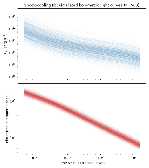
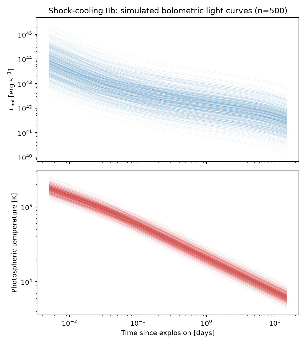
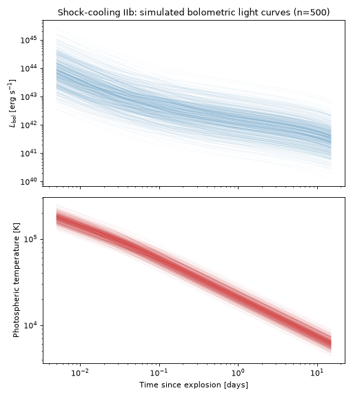
The plot below draws 500 random parameter realizations from the priors above and shows the resulting bolometric light curves and photospheric temperatures, using the default MoragShockCoolingSED. No comparison data is overlaid: unlike the other supernova populations in this package, there is not yet a curated bolometric/temperature dataset for shock-cooling Type IIb events under test_data/transients.

(Source code, png, hires.png, pdf)

---

Simulated UVOIR Light Curves (Rubin + UVEX)

Because the shock-cooling phase lasts only days, seeing it well requires a cadence much tighter than the multi-day cadences typically used for longer-lived transients. The two panels below show two random parameter realizations at a fixed redshift (\(z=0.02\), roughly 90 Mpc), each observed by Rubin (g/r/i, 30 s visits) and UVEX (FUV/NUV, 900 s visits) on a shared 12-hour cadence over the first 12 days: solid curves are the noiseless theory light curves, points are simulated photometry (shot noise plus, for Rubin, its own photometric-calibration floor), and open triangles are \(\mathrm{SNR}<5\) upper limits. This is meant to give a sense of what the model’s SEDs actually look like observationally, not a rate/yield forecast – see the other transient pages in this section for that kind of analysis.

(Source code)

References

[1] (1,2)

Jonathan Morag, Ido Irani, Nir Sapir, and Eli Waxman. Shock cooling emission from explosions of red supergiants: II. An analytic model of deviations from blackbody emission. \mnras , 528(4):7137–7155, March 2024. arXiv:2307.05598, doi:10.1093/mnras/stae374.

[2] (1,2)

Louis-Gregory Strolger, Tomas Dahlen, Steven A. Rodney, Or Graur, Adam G. Riess, Curtis McCully, Swara Ravindranath, Bahram Mobasher, and A. Kristin Shahady. The rate of core collapse supernovae to redshift 2.5 from the CANDELS and CLASH supernova surveys. The Astrophysical Journal, 813(2):93, 2015. arXiv:1509.06574, doi:10.1088/0004-637X/813/2/93.

[3]

Piero Madau and Mark Dickinson. Cosmic star-formation history. Annual Review of Astronomy and Astrophysics, 52:415–486, 2014. arXiv:1403.0007, doi:10.1146/annurev-astro-081811-125615.

[4] (1,2)

Isaac Shivvers, Maryam Modjaz, WeiKang Zheng, Yuqian Liu, Alexei V. Filippenko, Jeffrey M. Silverman, Thomas Matheson, Andrea Pastorello, Or Graur, Ryan J. Foley, Ryan Chornock, Nathan Smith, Jesse Leaman, and Stefano Benetti. Revisiting the lick observatory supernova search volume-limited sample: updated classifications and revised stripped-envelope supernova fractions. Publications of the Astronomical Society of the Pacific, 129(975):054201, 2017. arXiv:1609.02922, doi:10.1088/1538-3873/aa54a6.