Type I (Stripped-Envelope) Supernovae

Type Ib and Type Ic supernovae are core-collapse explosions of massive stars that lost their hydrogen envelope (Ib: helium remains; Ic: helium is also stripped) before exploding. Their light curves are powered by the radioactive decay of \(^{56}\mathrm{Ni}\) and are typically a single peak, roughly two to three weeks after explosion, followed by a decline; unlike Type IIb SNe (Type II Supernovae) they lack a distinct early shock-cooling peak. All three subtypes on this page – Ib, Ic and Ic-BL (broad-lined) – are modeled with the same first-principles Arnett-style radioactive-decay diffusion physics as Type Ia (ArnettDecaySED), differing only in their priors (and, for Ic-BL, in its higher characteristic ejecta velocities and kinetic energies); the three populations are implemented as sibling transient classes below.

Note

The Type Ib and Type Ic priors on M_Ni, M_ej and v_ej are the per-subtype sample statistics (mean, sample standard deviation) of the analytical Arnett-model fits in Table 6 of Lyman et al.[1] (13 Ib and 8 Ic events). kappa is fixed at the single value (\(0.06\,\mathrm{cm^2\,g^{-1}}\)) Lyman et al. 2016 themselves assume for every fit in their sample rather than fitting per event. kappa_gamma has no analogue in Lyman et al. 2016’s leakage-free formalism (the original Arnett 1982 diffusion model), so it is instead fixed at \(0.04\,\mathrm{cm^2\,g^{-1}}\), comparable to Type Ia’s Scalzo+14-derived value. Ib and Ic share this same construction and differ only in the subsample statistics and event rates. Type Ic-BL instead uses sample statistics of its own explosion-property table – see its tab below.

Type Ia

Type Ia supernovae are thermonuclear explosions of carbon-oxygen white dwarfs, not core-collapse events – there is no compact remnant and no massive-star progenitor, so neither this population’s SED nor its rate shares any machinery with the Type Ib/Ic/II populations elsewhere on this page. Their light curves are powered by the radioactive decay of \(^{56}\mathrm{Ni}\) synthesized in the explosion, following the same Arnett-style diffusion physics as the SLSNe-I model (Superluminous Supernovae (SLSNe-I)), but without a magnetar central engine.

Implemented by TypeIaSNe, pairing TypeIaSED with a delay-time-distribution rate (below) rather than a fixed fraction of the core-collapse rate.

Quick Facts

Quantity	Value	Source	Notes
Rate	Cosmic star formation history convolved with a power-law delay-time distribution (DTD); local rate \(\approx2.3\times10^{-5}\ \mathrm{Mpc^{-3}\,yr^{-1}}\) (\(\approx2.3\times10^{4}\ \mathrm{Gpc^{-3}\,yr^{-1}}\))	Maoz and Graur[2], Madau and Dickinson[3]	supernovae_Ia_rate(): DTD \(\Psi(\tau)\propto\tau^{-1.1}\) for \(\tau>40\) Myr, normalized to \(N_\mathrm{Ia}/M_\star=(1.3\pm0.1)\times10^{-3}\,M_\odot^{-1}\) (Maoz & Graur 2017), convolved with the Madau & Dickinson (2014) star formation history. Unlike the core-collapse subtypes’ instantaneous tracer, the broadly distributed delay times give SNe Ia a flatter, slower-declining rate shape at high redshift. The rate is exactly linear in \(N_\mathrm{Ia}/M_\star\), so RATE_CI (\(\pm7.7\%\)) is evaluated by calling supernovae_Ia_rate directly at that normalization’s \(\pm1\sigma\) endpoints, rather than assumed analytically – see Rate Uncertainty and All-Sky Yield.
Redshift limit	\(z = 1\)	–	Set from an actual sample_event_redshift/peak-apparent-magnitude check against the UVEX bandpasses (25 AB mag limiting-magnitude screen): no simulated event peaks above the limit beyond \(z\approx0.8\) in either band, and the NUV-detected fraction per redshift bin has already fallen to zero by \(z=1\).
Duration	365 days	–	Covers the rise to peak (median \(\approx14\) d after explosion) through the decline to \(10^{-3}\) of peak for nearly the whole prior (16th-84th percentile \(\approx270\)-\(325\) d, rest frame).

SED Model

Model Class: TypeIaSED

TypeIaSED reuses ArnettDecaySED’s Arnett-style radioactive-decay diffusion light curve and floored-photosphere blackbody entirely (the same \(L(t)\)/\(T(t)\) machinery documented for the SLSNe-I model in Superluminous Supernovae (SLSNe-I), but driven by \(^{56}\mathrm{Ni}\to{}^{56}\mathrm{Co}\to{}^{56}\mathrm{Fe}\) decay heating rather than magnetar spin-down):

\[F_\mathrm{decay}(t) = M_\mathrm{Ni}\left[\epsilon_\mathrm{Ni}\,e^{-t/\tau_\mathrm{Ni}} + \epsilon_\mathrm{Co}\left(e^{-t/\tau_\mathrm{Co}} - e^{-t/\tau_\mathrm{Ni}}\right)\right], \qquad T(t) = \max\left\{\left[\frac{L(t)}{4\pi\sigma_\mathrm{SB}(v_\mathrm{ej}t)^2}\right]^{1/4}, T_\mathrm{floor}\right\}.\]

The priors follow Sarin et al.[4] (a sample of 2205 SNe Ia from ZTF): M_Ni and M_ej are the population-level Gaussians from that paper’s hierarchical Arnett-model fit (\(\mu_\mathrm{Ni}=0.64\,M_\odot\), \(\sigma_\mathrm{Ni}=0.42\,M_\odot\); \(\mu_\mathrm{ej}=1.26\,M_\odot\), \(\sigma_\mathrm{ej}=0.33\,M_\odot\)), kappa_gamma is fixed at the value adopted by Scalzo et al.[5], and kappa is uniform over that paper’s marginalization range.

Parameter priors

Parameter	Symbol	Prior	Notes / Source
M_Ni	\(M_\mathrm{Ni}\)	TruncatedNormal(0.64, \(\sigma\)=0.42; bounds \([0.05, 3.0]\,M_\odot\))	Sarin et al.[4].
M_ej	\(M_\mathrm{ej}\)	TruncatedNormal(1.26, \(\sigma\)=0.33; bounds \([0.05, 3.0]\,M_\odot\))	Sarin et al.[4].
v_ej	\(v_\mathrm{ej}\)	Normal(11, \(\sigma\)=1) \(\times10^3\ \mathrm{km\,s^{-1}}\)	Sarin et al.[4].
kappa	\(\kappa\)	Uniform(0.05, 0.15) \(\mathrm{cm^2\,g^{-1}}\)	Marginalization-prior range, Sarin et al.[4].
kappa_gamma	\(\kappa_\gamma\)	Fixed, 0.03 \(\mathrm{cm^2\,g^{-1}}\)	Scalzo et al.[5].
T_floor	\(T_\mathrm{floor}\)	TruncatedNormal(6000 K, \(\sigma\)=1000 K; bounds \([3000, 10000]\) K)	Same floor as the other Arnett-based models on this site (see Superluminous Supernovae (SLSNe-I)); not calibrated against SNe Ia data specifically.

Simulated Light Curves

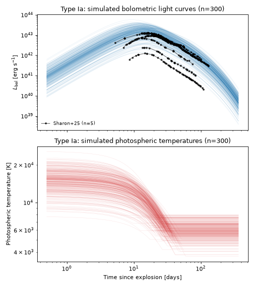
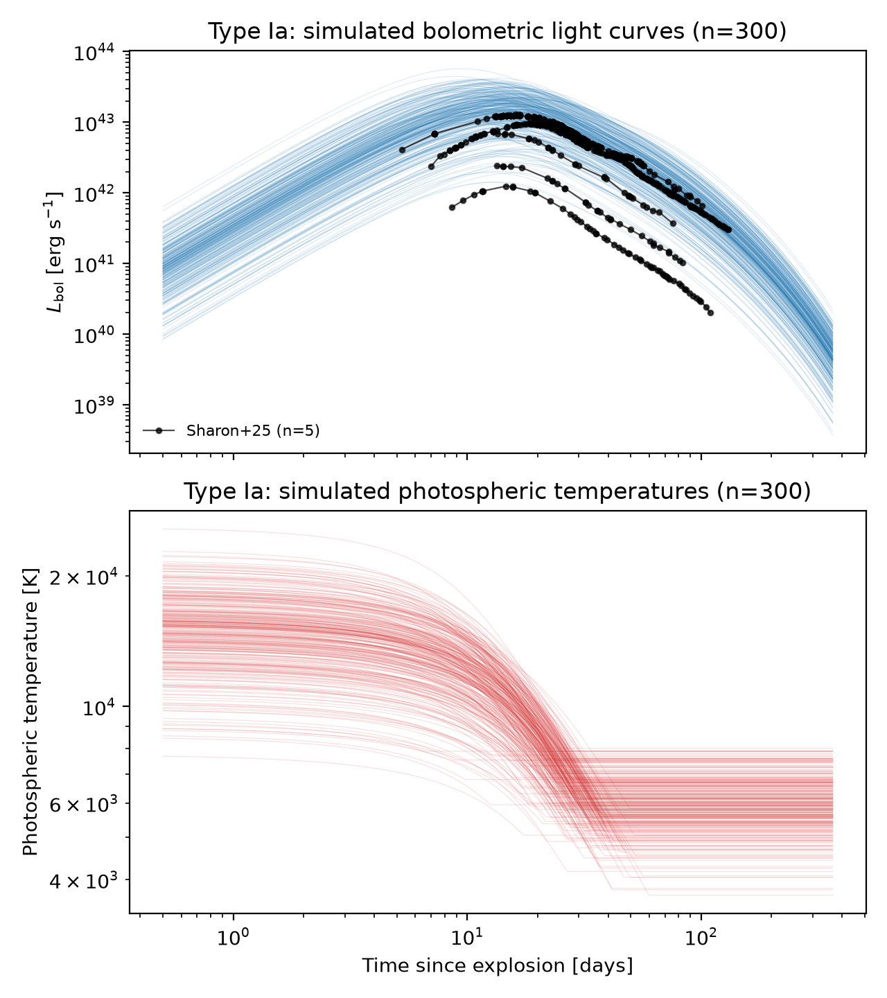
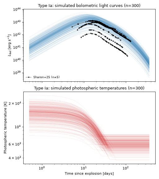
The plot below draws 300 random parameter realizations from the priors above and shows the resulting bolometric light curves and photospheric temperatures. The top panel is overlaid with the individual bolometric light curves (time since explosion) of the five Type Ia SNe of Sharon et al.[6]. No photospheric temperature data is bundled for Type Ia, so the bottom panel is unadorned.

(Source code, png, hires.png, pdf)

Observability Summary

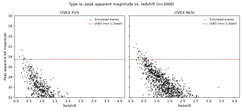
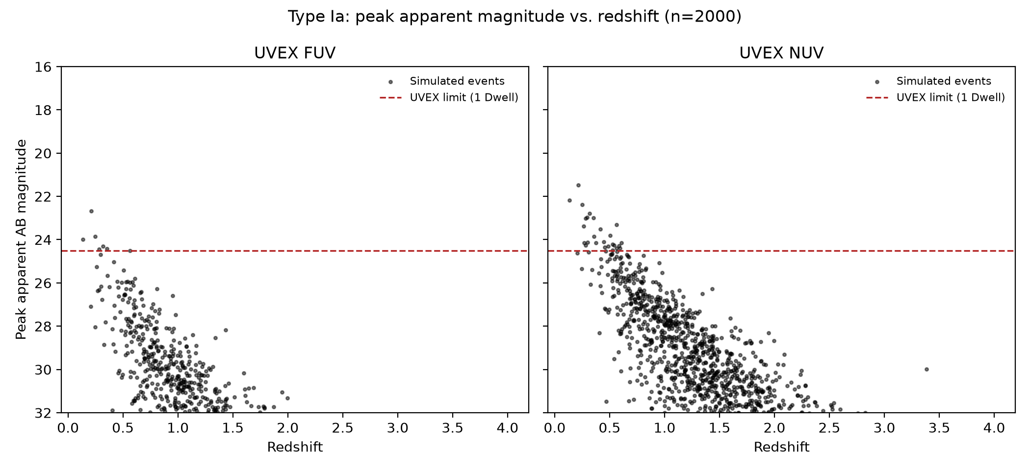
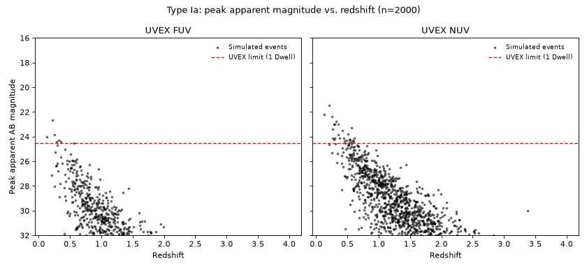
Below are the redshifts \(z\) and corresponding bandpass peak apparent AB magnitudes \(m_\mathrm{AB}\) of 2000 simulated events drawn from the priors above (with redshift_limit temporarily raised to 4 to show the falloff), with the UVEX 1 Dwell limit of \(m<24.5\) overplotted. This justifies the \(z=1\) redshift limit adopted above.

(Source code, png, hires.png, pdf)

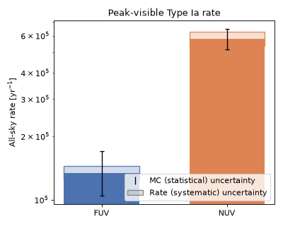
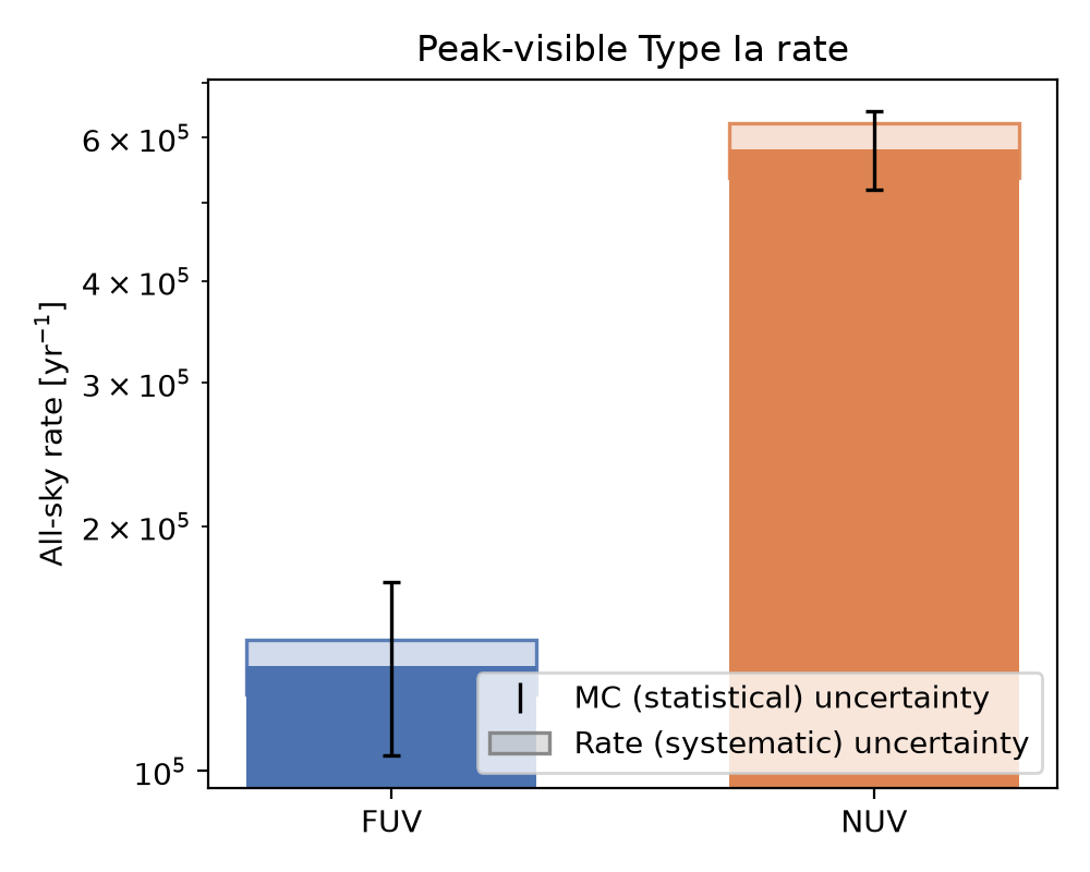
The anticipated rate of SNe Ia detectable by UVEX at this limit is as follows, assuming that any event above the \(m<24.5\) limit is detectable, and that the population is isotropic and homogeneous in comoving volume out to \(z=1\):

(Source code, png, hires.png, pdf)

Type Ib

Implemented by TypeIbSNe, pairing TypeIbSED with the rate/duration metadata described below.

Quick Facts

Quantity	Value	Source	Notes
Rate	\(R_\mathrm{CC}(z) = k\,\psi_\mathrm{UV}(z)\); Type Ib 10.8% of \(R_\mathrm{CC}(z)\)	Strolger et al.[7], Madau and Dickinson[3], Shivvers et al.[8]	Tracks the cosmic star-formation history. Shivvers et al.[8] find Ib is \(35.6\pm11.4\%\) of the stripped-envelope (SESNe) rate, which is itself \(30.4^{+5.0}_{-4.9}\%\) of the total core-collapse rate, so the Type Ib fraction is \(0.356\times0.304=0.108\). Combined in quadrature with Strolger et al.[7]’s \(+27\%/-31\%\) normalization uncertainty, this gives RATE_CI (see Rate Uncertainty and All-Sky Yield).
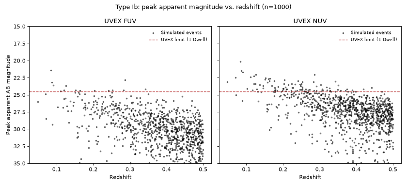
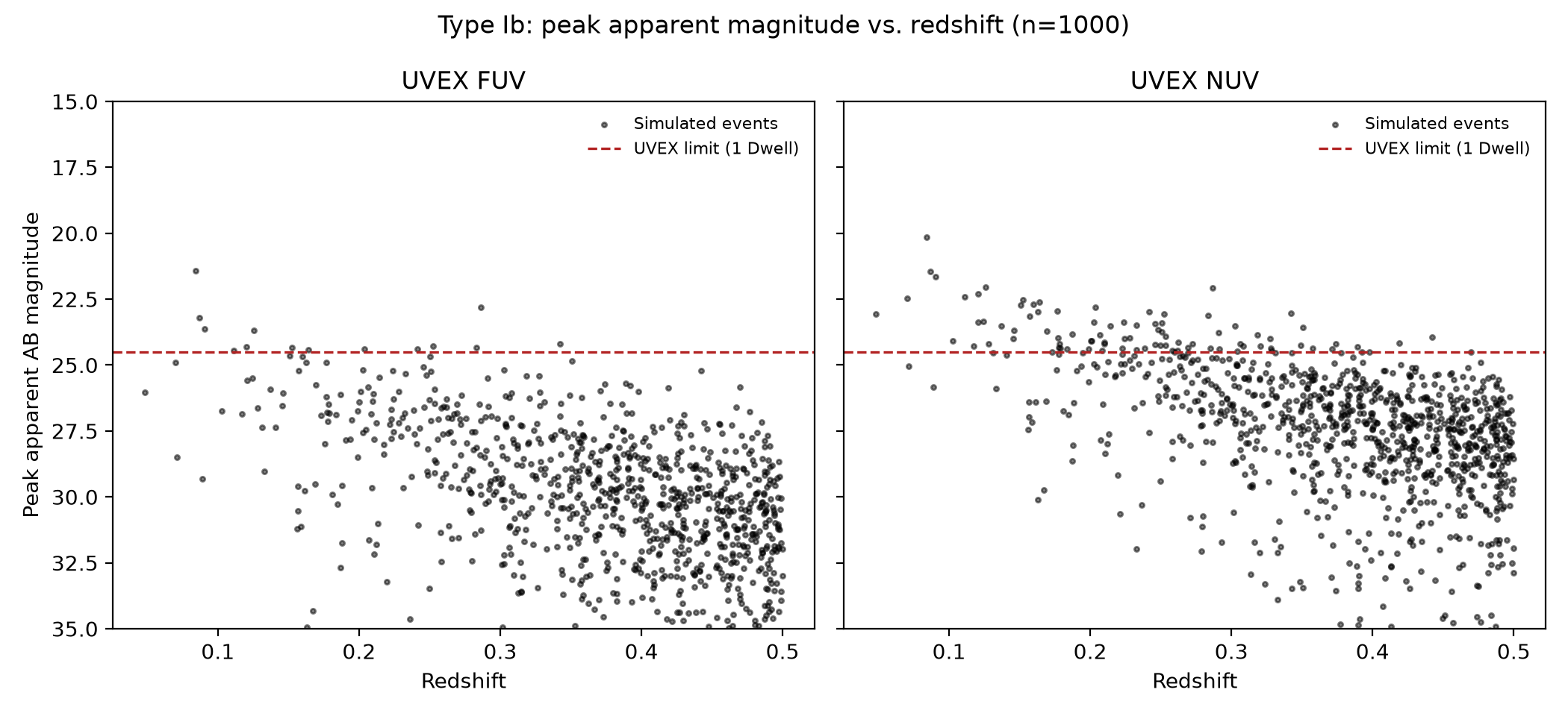
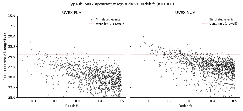
Redshift limit	\(z = 0.5\)	–	Below the Type IIP and IIb limits, since these events peak at lower luminosity and are cool in the UV: in the observability check below, no simulated event beyond \(z \approx 0.3\) clears the UVEX limit.
Duration	100 days	–	Covers the rise, peak (\(t_p \approx 16\) d after explosion, prior median) and the decline.

SED Model

Model Class: TypeIbSED

TypeIbSED reuses ArnettDecaySED’s Arnett-style radioactive-decay diffusion light curve and floored-photosphere blackbody entirely – the same \(L(t)\)/\(T(t)\) machinery documented for Type Ia above – with a single Ni-56 mass decaying through \(^{56}\mathrm{Ni}\to{}^{56}\mathrm{Co}\to{}^{56}\mathrm{Fe}\):

\[F_\mathrm{decay}(t) = M_\mathrm{Ni}\left[\epsilon_\mathrm{Ni}\,e^{-t/\tau_\mathrm{Ni}} + \epsilon_\mathrm{Co}\left(e^{-t/\tau_\mathrm{Co}} - e^{-t/\tau_\mathrm{Ni}}\right)\right], \qquad T(t) = \max\left\{\left[\frac{L(t)}{4\pi\sigma_\mathrm{SB}(v_\mathrm{ej}t)^2}\right]^{1/4}, T_\mathrm{floor}\right\}.\]

The priors on M_Ni, M_ej and v_ej are the SN Ib subsample statistics (mean, sample standard deviation) of the analytical-model fits in Table 6 of Lyman et al.[1] (13 events). kappa is fixed at \(0.06\,\mathrm{cm^2\,g^{-1}}\), the single grey optical opacity value that paper assumes (rather than fits) for every event in its sample. kappa_gamma is fixed at \(0.04\,\mathrm{cm^2\,g^{-1}}\), comparable to Type Ia’s Scalzo+14-derived value, since Lyman et al. 2016’s own analytical model has no gamma-ray leakage term at all (it is the original Arnett 1982 diffusion formalism) and so gives no direct constraint on it. T_floor is left close to Type Ia’s value.

Parameter priors

Parameter	Symbol	Prior	Notes / Source
M_Ni	\(M_\mathrm{Ni}\)	TruncatedNormal(0.17, \(\sigma\)=0.16; bounds \([0.01, 3.0]\,M_\odot\))	Lyman et al.[1], SN Ib subsample (13 events).
M_ej	\(M_\mathrm{ej}\)	TruncatedNormal(2.6, \(\sigma\)=1.1; bounds \([0.1, 8.0]\,M_\odot\))	Lyman et al.[1], SN Ib subsample.
v_ej	\(v_\mathrm{ej}\)	TruncatedNormal(9.9, \(\sigma\)=1.4; bounds \([4, 16]\times10^3\ \mathrm{km\,s^{-1}}\))	Lyman et al.[1], SN Ib subsample photospheric velocities.
kappa	\(\kappa\)	Fixed, 0.06 \(\mathrm{cm^2\,g^{-1}}\)	Lyman et al.[1]’s assumed (not fit) value.
kappa_gamma	\(\kappa_\gamma\)	Fixed, 0.04 \(\mathrm{cm^2\,g^{-1}}\)	Not constrained by Lyman et al.[1] (no leakage term in their model); comparable to Type Ia’s Scalzo et al.[5] value.
T_floor	\(T_\mathrm{floor}\)	TruncatedNormal(5000 K, \(\sigma\)=1000 K; bounds \([3000, 10000]\) K)	Same floor family as the other Arnett-based models on this site; not calibrated against Ib data specifically.

Simulated Light Curves

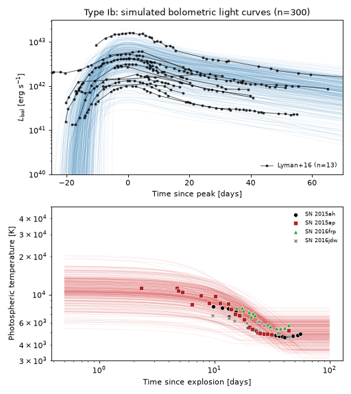
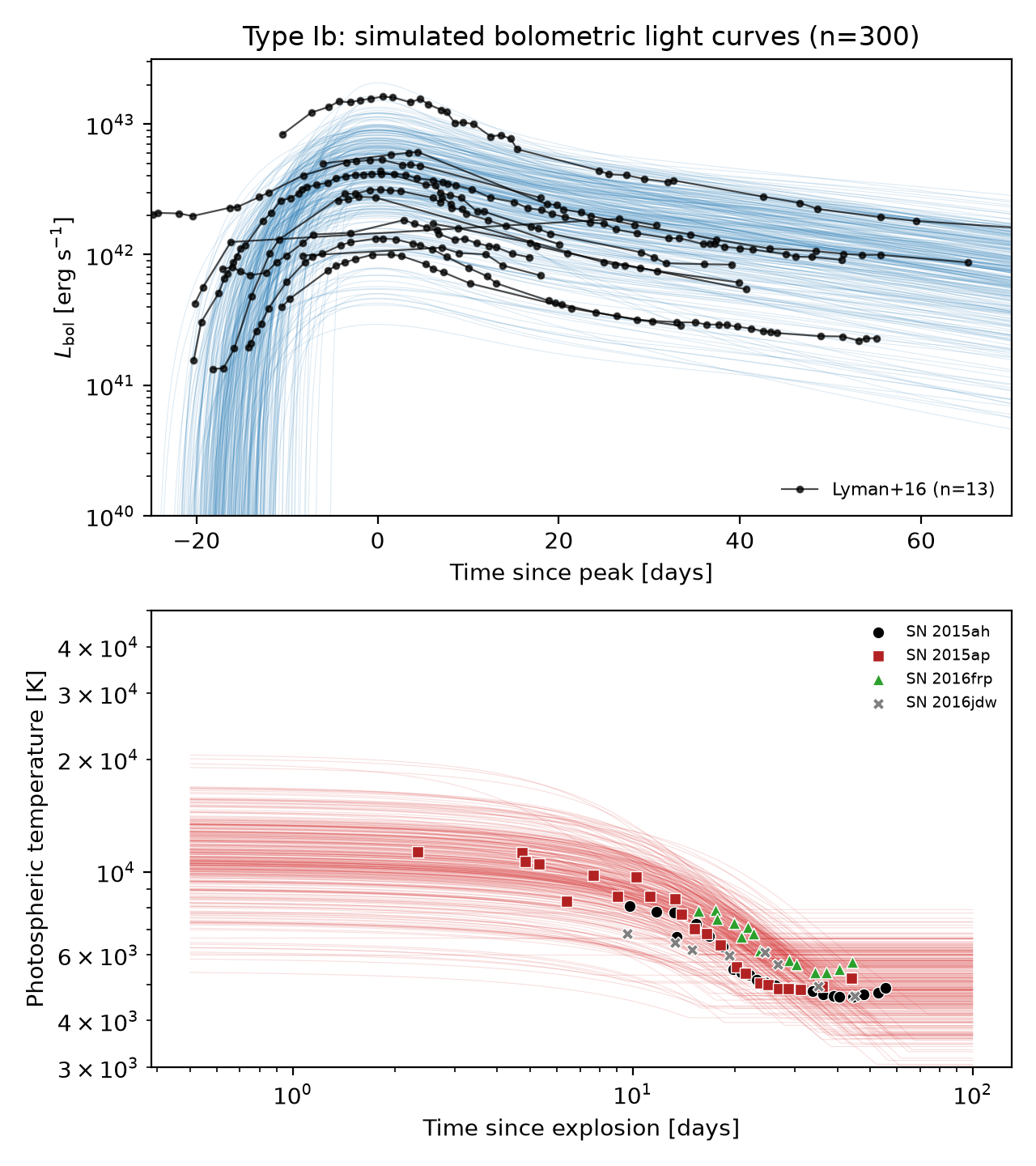
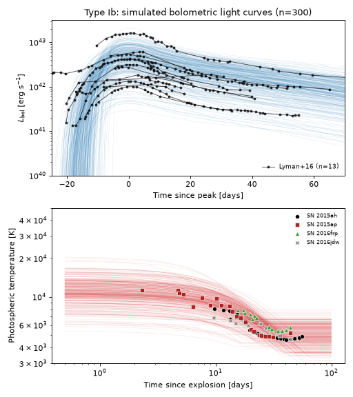
The plot below draws 300 random parameter realizations from the priors above. The top panel shows the bolometric light curves, each shifted so that its own peak sits at zero, overlaid with the individual bolometric light curves of the Type Ib SNe in Lyman et al.[1], which are measured relative to maximum light; this checks the shape of the light curve (rise, peak width and decline) predicted by the Arnett diffusion model against the same sample its priors are drawn from. The bottom panel shows the floored-photosphere blackbody temperature against time since explosion, overlaid with the temperatures of the Type Ib SNe in Prentice et al.[9], shifted to time since explosion using the tabulated \(t_p\).

(Source code, png, hires.png, pdf)

Observability Summary

Below are the redshifts \(z\) and corresponding bandpass peak apparent AB magnitudes \(m_\mathrm{AB}\) of 1000 simulated events drawn from the priors above, with the UVEX 1 Dwell limit of \(m<24.5\) overplotted.

(Source code, png, hires.png, pdf)

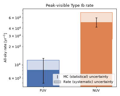
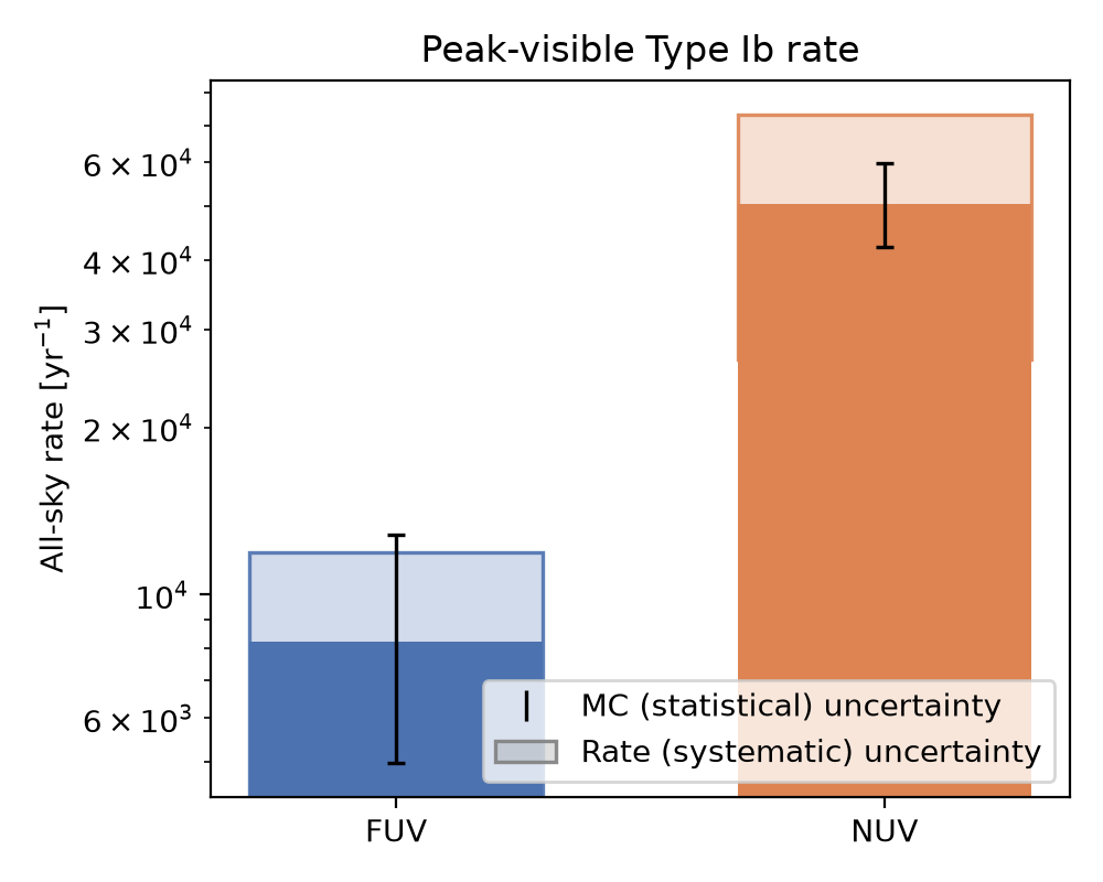
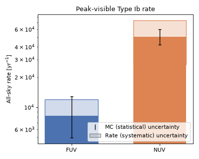
The anticipated rate detectable by UVEX at this limit is as follows, assuming that any event above the \(m<24.5\) limit is detectable, and that the population is isotropic and homogeneous in comoving volume out to its redshift limit:

(Source code, png, hires.png, pdf)

Type Ic

Implemented by TypeIcSNe, pairing TypeIcSED with the rate/duration metadata described below.

Quick Facts

Quantity	Value	Source	Notes
Rate	\(R_\mathrm{CC}(z) = k\,\psi_\mathrm{UV}(z)\); Type Ic 6.5% of \(R_\mathrm{CC}(z)\)	Strolger et al.[7], Madau and Dickinson[3], Shivvers et al.[8]	Tracks the cosmic star-formation history. Shivvers et al.[8] find Ic is \(21.5\pm8.6\%\) of the stripped-envelope (SESNe) rate, which is itself \(30.4^{+5.0}_{-4.9}\%\) of the total core-collapse rate, so the Type Ic fraction is \(0.215\times0.304=0.065\). Combined in quadrature with Strolger et al.[7]’s \(+27\%/-31\%\) normalization uncertainty, this gives RATE_CI (see Rate Uncertainty and All-Sky Yield).
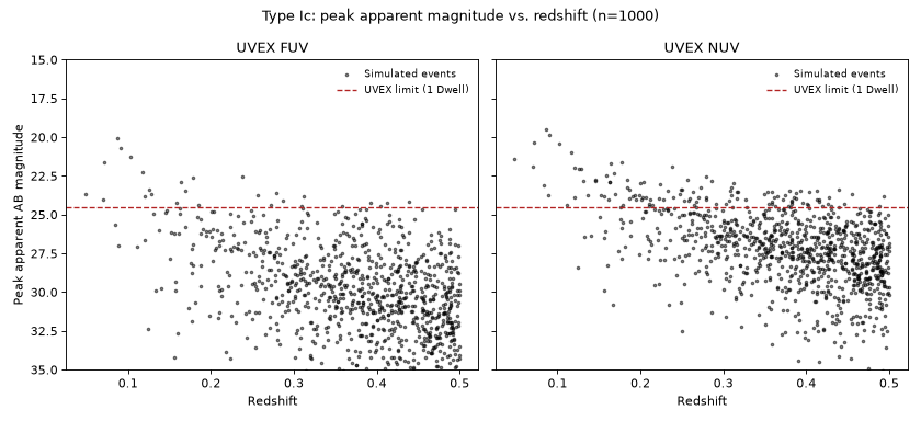
Redshift limit	\(z = 0.5\)	–	Below the Type IIP and IIb limits, since these events peak at lower luminosity and are cool in the UV: in the observability check below, no simulated event beyond \(z \approx 0.5\) clears the UVEX limit.
Duration	100 days	–	Covers the rise, peak (\(t_p \approx 17\) d after explosion, prior median) and the decline.

SED Model

Model Class: TypeIcSED

TypeIcSED shares its construction entirely with Type Ib’s TypeIbSED (see its SED Model section above for the \(F_\mathrm{decay}(t)\)/\(T(t)\) math and the reasoning behind kappa, kappa_gamma and T_floor), differing only in that M_Ni, M_ej and v_ej are drawn from the SN Ic subsample statistics of Table 6 of Lyman et al.[1] (8 events) instead of the Type Ib ones.

Parameter priors

Parameter	Symbol	Prior	Notes / Source
M_Ni	\(M_\mathrm{Ni}\)	TruncatedNormal(0.22, \(\sigma\)=0.16; bounds \([0.01, 3.0]\,M_\odot\))	Lyman et al.[1], SN Ic subsample (8 events).
M_ej	\(M_\mathrm{ej}\)	TruncatedNormal(3.0, \(\sigma\)=2.8; bounds \([0.1, 6.0]\,M_\odot\))	Lyman et al.[1], SN Ic subsample.
v_ej	\(v_\mathrm{ej}\)	TruncatedNormal(10.4, \(\sigma\)=1.2; bounds \([4, 16]\times10^3\ \mathrm{km\,s^{-1}}\))	Lyman et al.[1], SN Ic subsample photospheric velocities.
kappa	\(\kappa\)	Fixed, 0.06 \(\mathrm{cm^2\,g^{-1}}\)	Lyman et al.[1]’s assumed (not fit) value.
kappa_gamma	\(\kappa_\gamma\)	Fixed, 0.04 \(\mathrm{cm^2\,g^{-1}}\)	Not constrained by Lyman et al.[1] (no leakage term in their model); comparable to Type Ia’s Scalzo et al.[5] value.
T_floor	\(T_\mathrm{floor}\)	TruncatedNormal(6000 K, \(\sigma\)=1000 K; bounds \([3000, 10000]\) K)	Same floor family as the other Arnett-based models on this site; not calibrated against Ic data specifically.

Simulated Light Curves

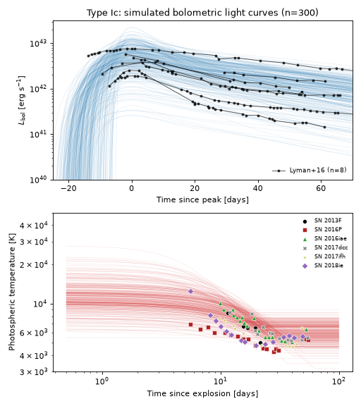
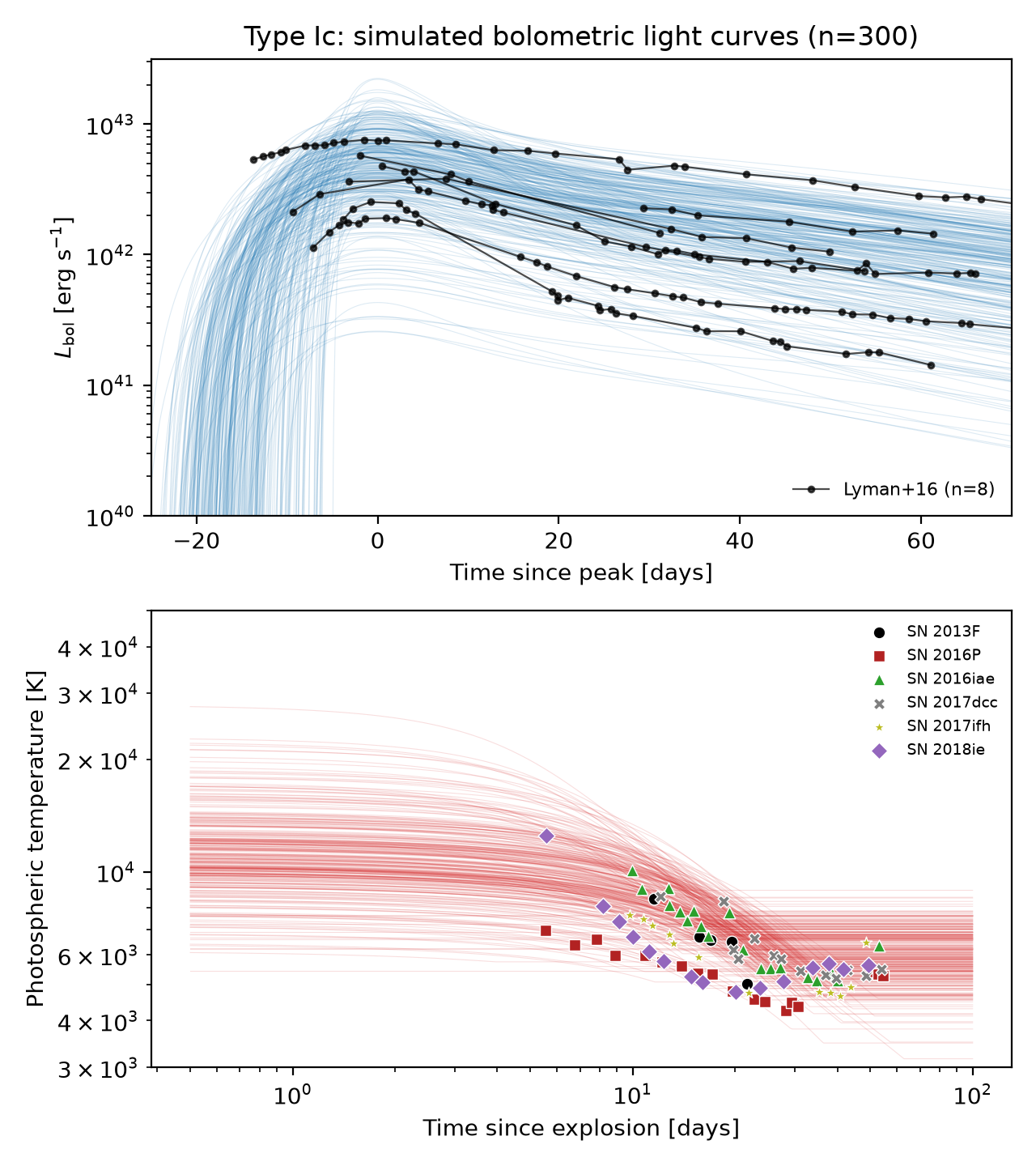
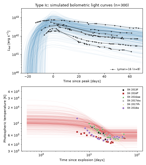
The plot below draws 300 random parameter realizations from the priors above. The top panel shows the bolometric light curves, each shifted so that its own peak sits at zero, overlaid with the individual bolometric light curves of the Type Ic SNe in Lyman et al.[1], which are measured relative to maximum light; this checks the shape of the light curve (rise, peak width and decline) predicted by the Arnett diffusion model against the same sample its priors are drawn from. The bottom panel shows the floored-photosphere blackbody temperature against time since explosion, overlaid with the temperatures of the Type Ic SNe in Prentice et al.[9], shifted to time since explosion using the tabulated \(t_p\).

(Source code, png, hires.png, pdf)

Observability Summary

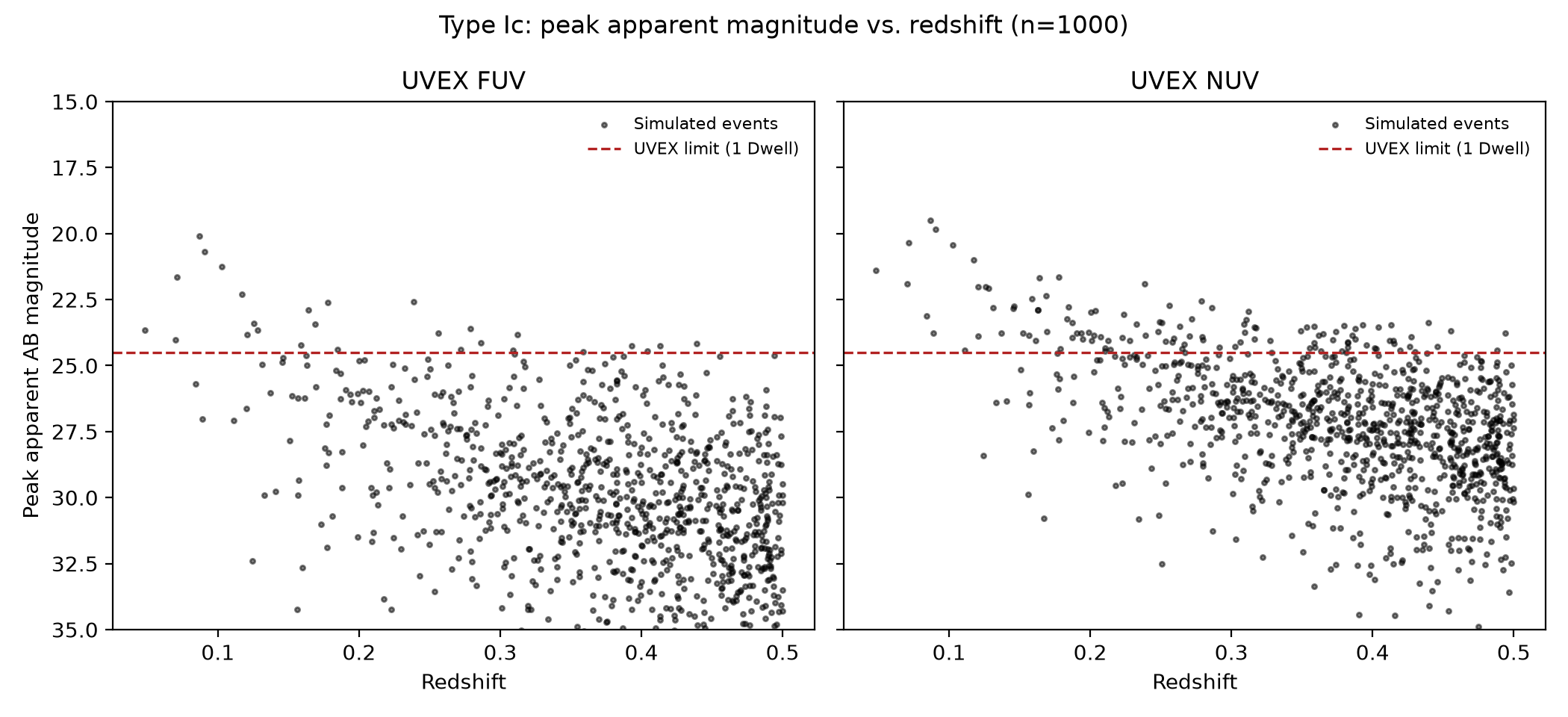
Below are the redshifts \(z\) and corresponding bandpass peak apparent AB magnitudes \(m_\mathrm{AB}\) of 1000 simulated events drawn from the priors above, with the UVEX 1 Dwell limit of \(m<24.5\) overplotted.

(Source code, png, hires.png, pdf)

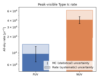
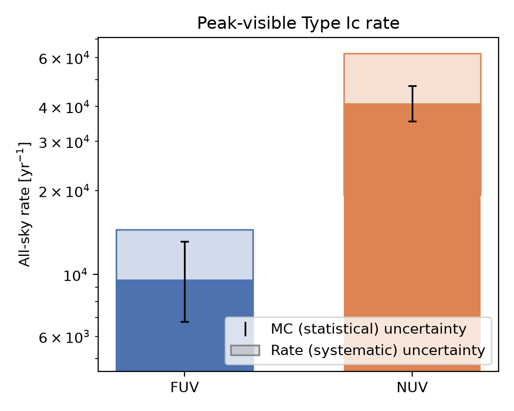
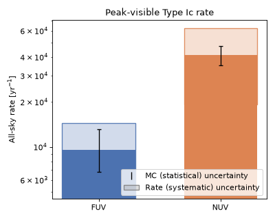
The anticipated rate detectable by UVEX at this limit is as follows, assuming that any event above the \(m<24.5\) limit is detectable, and that the population is isotropic and homogeneous in comoving volume out to its redshift limit:

(Source code, png, hires.png, pdf)

Type Ic-BL

Type Ic-BL (broad-lined) supernovae are Type Ic explosions with unusually high kinetic energies and ejecta velocities, identified spectroscopically by their broad, blended absorption features. Like Type Ib/Type Ic above and Type Ia, this population’s SED follows the same first-principles Arnett-style radioactive-decay model, but with its own priors, calibrated from an explosion-property table (nickel mass, ejecta mass, photospheric velocity) specific to its own ZTF sample rather than the Lyman et al. 2016 sample used for Type Ib/Type Ic.

Implemented by TypeIcBLSNe, pairing TypeIcBLSED with the rate/duration metadata described below.

Quick Facts

Quantity	Value	Source	Notes
Rate	\(R_\mathrm{CC}(z) = k\,\psi_\mathrm{UV}(z)\); Type Ic-BL 1.1% of \(R_\mathrm{CC}(z)\)	Strolger et al.[7], Madau and Dickinson[3], Shivvers et al.[8]	Tracks the cosmic star-formation history. Shivvers et al.[8] find Ic-BL is \(3.7^{+2.9}_{-3.7}\%\) of the stripped-envelope (SESNe) rate, which is itself \(30.4^{+5.0}_{-4.9}\%\) of the total core-collapse rate, so the Type Ic-BL fraction is \(0.037\times0.304=0.0112\). Combined in quadrature with Strolger et al.[7]’s \(+27\%/-31\%\) normalization uncertainty, this gives RATE_CI (see Rate Uncertainty and All-Sky Yield). The lower bound on the Ic-BL-of-SESNe fraction is itself consistent with zero, so the combined lower RATE_CI factor is slightly negative; treat the lower bound as effectively zero rather than literally.
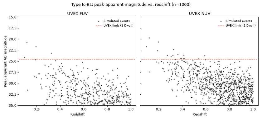
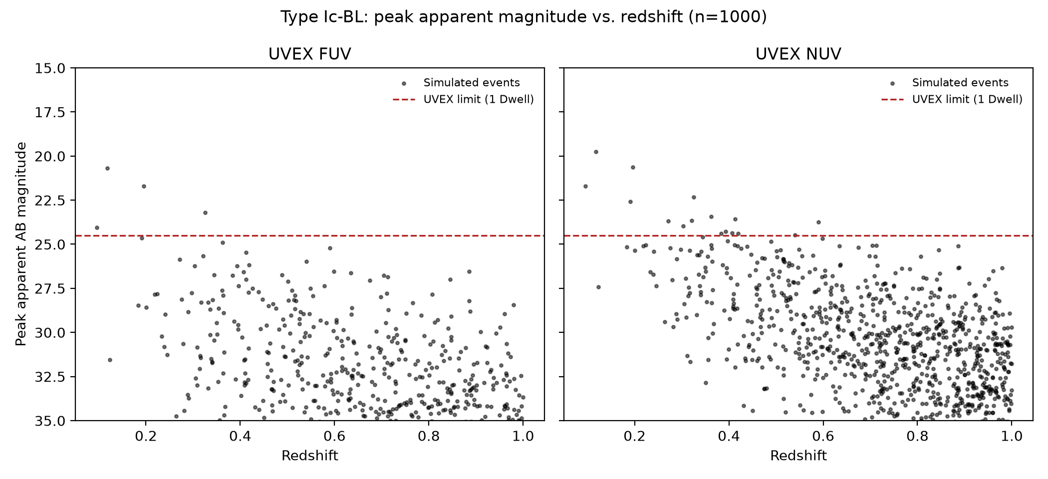
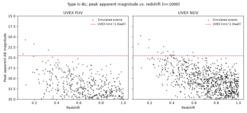
Redshift limit	\(z = 1\)	–	Wider than the Type Ib/Type Ic limit, to cover this population’s higher ejecta velocities and kinetic energies; in the observability check below, no simulated event beyond \(z \approx 0.55\) clears the UVEX limit.
Duration	100 days	–	Covers the rise, peak and decline, matching Type Ib/Type Ic.

SED Model

Model Class: TypeIcBLSED

TypeIcBLSED reuses ArnettDecaySED’s Arnett-style radioactive-decay diffusion light curve and floored-photosphere blackbody entirely (the same \(L(t)\)/\(T(t)\) machinery documented for Type Ia above and for the SLSNe-I model in Superluminous Supernovae (SLSNe-I)):

\[F_\mathrm{decay}(t) = M_\mathrm{Ni}\left[\epsilon_\mathrm{Ni}\,e^{-t/\tau_\mathrm{Ni}} + \epsilon_\mathrm{Co}\left(e^{-t/\tau_\mathrm{Co}} - e^{-t/\tau_\mathrm{Ni}}\right)\right], \qquad T(t) = \max\left\{\left[\frac{L(t)}{4\pi\sigma_\mathrm{SB}(v_\mathrm{ej}t)^2}\right]^{1/4}, T_\mathrm{floor}\right\}.\]

The priors on M_Ni, M_ej and v_ej are sample statistics (mean, sample standard deviation) of the 36-event explosion-property table of Srinivasaragavan et al.[10] (nickel mass, kinetic energy, ejecta mass and photospheric velocity per event). One event (SN 2020wgz), whose reported \(M_\mathrm{Ni}=2.46\,M_\odot\) is a >5-sigma outlier driven by an e_k/m_ej lower limit rather than a measurement, is excluded from the M_Ni statistics; M_ej uses only rows with a measured (non-lower-limit) value; v_ej is identified with the sample’s photospheric velocities (v_ph), regardless of the epoch quoted. kappa and T_floor are not constrained by that table and are left at Type Ia’s values; kappa_gamma is instead fixed at a large value (full gamma-ray trapping across the simulated window), unlike Type Ia’s Scalzo+14 value.

Parameter priors

Parameter	Symbol	Prior	Notes / Source
M_Ni	\(M_\mathrm{Ni}\)	TruncatedNormal(0.33, \(\sigma\)=0.24; bounds \([0.02, 2.0]\,M_\odot\))	Srinivasaragavan et al.[10] (SN 2020wgz excluded, see above).
M_ej	\(M_\mathrm{ej}\)	TruncatedNormal(2.54, \(\sigma\)=1.95; bounds \([0.1, 10.0]\,M_\odot\))	Srinivasaragavan et al.[10], measured (non-lower-limit) rows only.
v_ej	\(v_\mathrm{ej}\)	TruncatedNormal(20.1, \(\sigma\)=4.96; bounds \([5, 45]\times10^3\ \mathrm{km\,s^{-1}}\))	Sample photospheric velocities (v_ph).
kappa	\(\kappa\)	Uniform(0.05, 0.15) \(\mathrm{cm^2\,g^{-1}}\)	Not constrained by the table; same range as Type Ia.
kappa_gamma	\(\kappa_\gamma\)	Fixed, 1000 \(\mathrm{cm^2\,g^{-1}}\)	Approximates full gamma-ray trapping across the simulated window; unlike Type Ia, not Scalzo et al.[5]’s value.
T_floor	\(T_\mathrm{floor}\)	TruncatedNormal(6000 K, \(\sigma\)=1000 K; bounds \([3000, 10000]\) K)	Same floor as the other Arnett-based models on this site; not calibrated against Ic-BL data specifically.

Simulated Light Curves

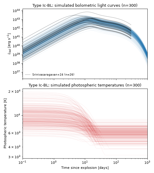
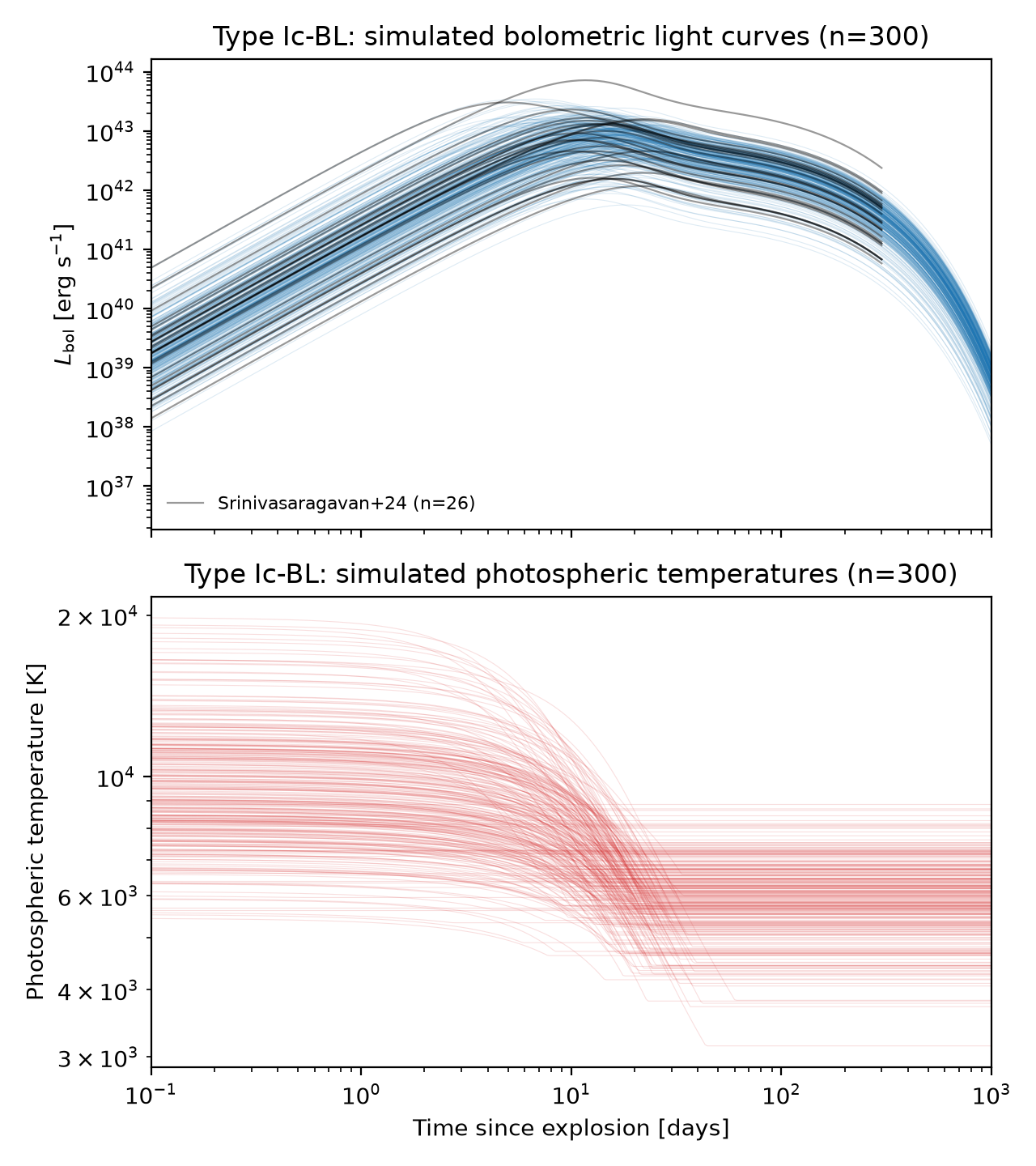
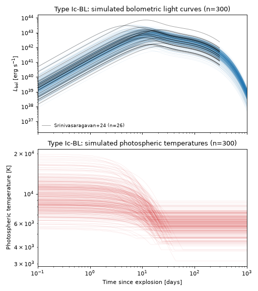
The plot below draws 300 random parameter realizations from the priors above and shows the resulting bolometric light curves and photospheric temperatures. The top panel is overlaid with the individual bolometric light curves (time since explosion) of the 26 Type Ic-BL SNe of Srinivasaragavan et al.[10] with a full explosion-property fit (the same sample the priors above are derived from). No photospheric temperature data is bundled for Type Ic-BL, so the bottom panel is unadorned.

(Source code, png, hires.png, pdf)

Observability Summary

Below are the redshifts \(z\) and corresponding bandpass peak apparent AB magnitudes \(m_\mathrm{AB}\) of 1000 simulated events drawn from the priors above, with the UVEX 1 Dwell limit of \(m<24.5\) overplotted.

(Source code, png, hires.png, pdf)

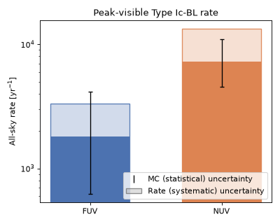
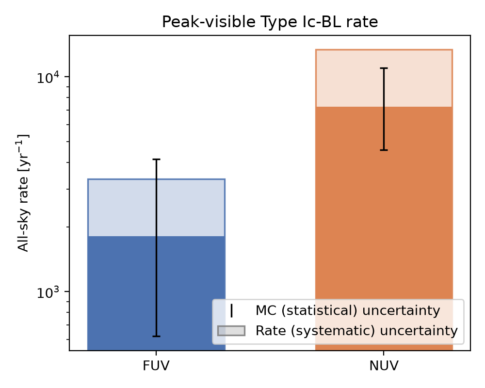
The anticipated rate detectable by UVEX at this limit is as follows, assuming that any event above the \(m<24.5\) limit is detectable, and that the population is isotropic and homogeneous in comoving volume out to its redshift limit:

(Source code, png, hires.png, pdf)

References

[1] (1,2,3,4,5,6,7,8,9,10,11,12,13,14,15)

J. D. Lyman, D. Bersier, P. A. James, P. A. Mazzali, J. J. Eldridge, M. Fraser, and E. Pian. Bolometric light curves and explosion parameters of 38 stripped-envelope core-collapse supernovae. Monthly Notices of the Royal Astronomical Society, 457:328–350, 2016. arXiv:1512.03422, doi:10.1093/mnras/stv2983.

[2]

Dan Maoz and Or Graur. Star Formation, Supernovae, Iron, and \ensuremath \alpha : Consistent Cosmic and Galactic Histories. \apj , 848(1):25, October 2017. arXiv:1703.04540, doi:10.3847/1538-4357/aa8b6e.

[3] (1,2,3,4)

Piero Madau and Mark Dickinson. Cosmic star-formation history. Annual Review of Astronomy and Astrophysics, 52:415–486, 2014. arXiv:1403.0007, doi:10.1146/annurev-astro-081811-125615.

[4] (1,2,3,4,5)

Nikhil Sarin, Ellen Lindsjö, Lisa Kelsey, Matthew Grayling, Jesper Sollerman, Steve Schulze, Adam A. Miller, Madeleine Ginolin, Erin E. Hayes, Conor M. B. Omand, Kaisey S. Mandel, Aaron Do, Suhail Dhawan, and Joel Johansson. Lightcurve Modelling of 2,205 ZTF DR2 Type Ia Supernovae: Implications for SN Ia Physics and Cosmology. \mnras , September 2026. arXiv:2602.02677, doi:10.1093/mnras/stag1739.

[5] (1,2,3,4,5)

R. Scalzo, G. Aldering, P. Antilogus, C. Aragon, S. Bailey, C. Baltay, S. Bongard, C. Button, F. Cellier-Holzem, M. Childress, N. Chotard, Y. Copin, H. K. Fakhouri, E. Gangler, J. Guy, A. Kim, M. Kowalski, M. Kromer, J. Nordin, P. Nugent, K. Paech, R. Pain, E. Pecontal, R. Pereira, S. Perlmutter, D. Rabinowitz, M. Rigault, K. Runge, C. Saunders, S. A. Sim, G. Smadja, C. Tao, S. Taubenberger, R. C. Thomas, and B. A. Weaver. Type ia supernova bolometric light curves and ejected mass estimates from the nearby supernova factory. Monthly Notices of the Royal Astronomical Society, 440(2):1498–1518, 2014. arXiv:1402.6842, doi:10.1093/mnras/stu350.

[6]

Amir Sharon, Doron Kushnir, and Nahliel Wygoda. All known Type Ia supernovae models fail to reproduce the observed bolometric luminosity–width correlation. \mnras , 540(4):3247–3262, July 2025. arXiv:2407.06859, doi:10.1093/mnras/staf808.

[7] (1,2,3,4,5,6)

Louis-Gregory Strolger, Tomas Dahlen, Steven A. Rodney, Or Graur, Adam G. Riess, Curtis McCully, Swara Ravindranath, Bahram Mobasher, and A. Kristin Shahady. The rate of core collapse supernovae to redshift 2.5 from the CANDELS and CLASH supernova surveys. The Astrophysical Journal, 813(2):93, 2015. arXiv:1509.06574, doi:10.1088/0004-637X/813/2/93.

[8] (1,2,3,4,5,6)

Isaac Shivvers, Maryam Modjaz, WeiKang Zheng, Yuqian Liu, Alexei V. Filippenko, Jeffrey M. Silverman, Thomas Matheson, Andrea Pastorello, Or Graur, Ryan J. Foley, Ryan Chornock, Nathan Smith, Jesse Leaman, and Stefano Benetti. Revisiting the lick observatory supernova search volume-limited sample: updated classifications and revised stripped-envelope supernova fractions. Publications of the Astronomical Society of the Pacific, 129(975):054201, 2017. arXiv:1609.02922, doi:10.1088/1538-3873/aa54a6.

[9] (1,2)

S. J. Prentice, C. Ashall, P. A. James, L. Short, P. A. Mazzali, D. Bersier, P. A. Crowther, C. Barbarino, T.-W. Chen, C. M. Copperwheat, M. J. Darnley, L. Denneau, N. Elias-Rosa, M. Fraser, L. Galbany, A. Gal-Yam, J. Harmanen, D. A. Howell, G. Hosseinzadeh, C. Inserra, E. Kankare, E. Karamehmetoglu, G. P. Lamb, M. Limongi, K. Maguire, C. McCully, F. Olivares E., A. S. Piascik, G. Pignata, D. E. Reichart, A. Rest, T. Reynolds, Ó. Rodríguez, J. L. O. Saario, S. Schulze, S. J. Smartt, K. W. Smith, J. Sollerman, B. Stalder, M. Sullivan, F. Taddia, S. Valenti, S. D. Vergani, S. C. Williams, and D. R. Young. Investigating the properties of stripped-envelope supernovae; what are the implications for their progenitors? Monthly Notices of the Royal Astronomical Society, 485(2):1559–1578, 2019. arXiv:1812.03716, doi:10.1093/mnras/sty3399.

[10] (1,2,3,4)

Gokul P. Srinivasaragavan, Sheng Yang, Shreya Anand, Jesper Sollerman, Anna Y. Q. Ho, Alessandra Corsi, S. Bradley Cenko, Daniel Perley, Steve Schulze, Marquice Sanchez-Fleming, Jack Pope, Nikhil Sarin, Conor Omand, Kaustav K. Das, Christoffer Fremling, Igor Andreoni, Rachel Bruch, Kevin B. Burdge, Kishalay De, Avishay Gal-Yam, Anjasha Gangopadhyay, Matthew J. Graham, Jacob E. Jencson, Viraj Karambelkar, Mansi M. Kasliwal, S. R. Kulkarni, Julia Martikainen, Yashvi S. Sharma, Anastasios Tzanidakis, Lin Yan, Yuhan Yao, Eric C. Bellm, Steven L. Groom, Frank J. Masci, Guy Nir, Josiah Purdum, Roger Smith, and Niharika Sravan. Optical and radio analysis of systematically classified broad-lined type ic supernovae from the zwicky transient facility. The Astrophysical Journal, 2024. arXiv:2408.14586.