Superluminous Supernovae (SLSNe-I)

Superluminous supernovae (SLSNe) reach peak luminosities roughly ten times higher than ordinary core-collapse or Type Ia supernovae and stay bright for weeks to months. The hydrogen-poor subclass, SLSNe-I, is the best studied: radioactive \(^{56}\mathrm{Ni}\) decay alone cannot supply enough energy to power most of these events, and their bright, blue, slowly-declining light curves are instead widely explained by the spin-down power of a newly formed, rapidly-rotating, strongly-magnetized neutron star (a magnetar) embedded in the expanding ejecta [1][2].

This population is implemented by MagnetarSLSNe, pairing ArnettMagnetarSpindownSED with the rate/duration metadata described below. Unlike the purely phenomenological SED shapes used elsewhere in this package, this SED is a semi-analytic solution of the underlying diffusion physics (Arnett[3], extended by Nicholl et al.[4] and Wang et al.[5]), so it is grouped with the other detailed physical models.

Quick Facts

Quantity	Value	Source	Notes
Rate	\(R_\mathrm{CC}(z) = k\,\psi_\mathrm{UV}(z)\); SLSN-I \(1/3500\) of \(R_\mathrm{CC}(z)\) (\(\approx18\ \mathrm{Gpc^{-3}\,yr^{-1}}\) locally)	Strolger et al.[6], Madau and Dickinson[7], Frohmaier et al.[8]	Frohmaier et al.[8] measure a local ratio of SLSN-I to all core-collapse SNe of \(1/3500^{+2800}_{-720}\) (uncertainty on the denominator, i.e. the rate itself spans \(1/6300\) to \(1/2780\)). Adopted as a constant fraction of the core-collapse rate, so it tracks the same star-formation history. Combined in quadrature with Strolger et al.[6]’s \(+27\%/-31\%\) normalization uncertainty, this gives RATE_CI (see Rate Uncertainty and All-Sky Yield).
Redshift limit	\(z = 4\)	–	Set from an actual generate_events/filter_by_snr run against the default UVEX schedule (25 AB mag limiting-magnitude screen, SNR \(>5\)).
Duration	600 days	–	Covers the rise (median \(\approx30\) d) and most of the decline. The bolometric light curve falls to \(10^{-3}\) of peak after a median of \(\approx540\) d (16th-84th percentile 250-1400 d, rest frame), so the slowest events’ faint tails are truncated by this window rather than fully simulated.

SED Model

Model Class: ArnettMagnetarSpindownSED

The SED model for the SLSNe-I population utilizes the standard Arnett-style diffusion[4] model driven by a magnetar spin-down power source.

The magnetar’s total rotation energy and spin-down timescale are[4]

\[E_\mathrm{mag} = 2.6\times10^{52}\left(\frac{M_\mathrm{NS}}{1.4\,M_\odot}\right)^{3/2}\left(\frac{P}{1\,\mathrm{ms}}\right)^{-2}\ \mathrm{erg},\]

and

\[t_\mathrm{mag} = 1.3\times10^{5}\left(\frac{M_\mathrm{NS}}{1.4\,M_\odot}\right)^{3/2}\left(\frac{P}{1\,\mathrm{ms}}\right)^{2}\left(\frac{B_\perp}{10^{14}\,\mathrm{G}}\right)^{-2}\ \mathrm{s}.\]

We therefore adopt the engine power source

\[F_\mathrm{mag}(t) = \frac{E_\mathrm{mag}}{t_\mathrm{mag}}\left(1 + \frac{t}{t_\mathrm{mag}}\right)^{-2}.\]

The resulting bolometric lightcurve, including leakage, is

\[L(t) = e^{-(t/t_d)^2}\left(1 - e^{-A/t^2}\right) \int_0^t 2 F_\mathrm{mag}(t')\,\frac{t'}{t_d}\,e^{(t'/t_d)^2}\,\frac{dt'}{t_d},\]

where

\[t_d = \sqrt{\frac{2\kappa M_\mathrm{ej}}{\beta c\,v_\mathrm{ej}}}\]

is the photon diffusion time and

\[A = \frac{3\kappa_\gamma M_\mathrm{ej}}{4\pi v_\mathrm{ej}^2},\]

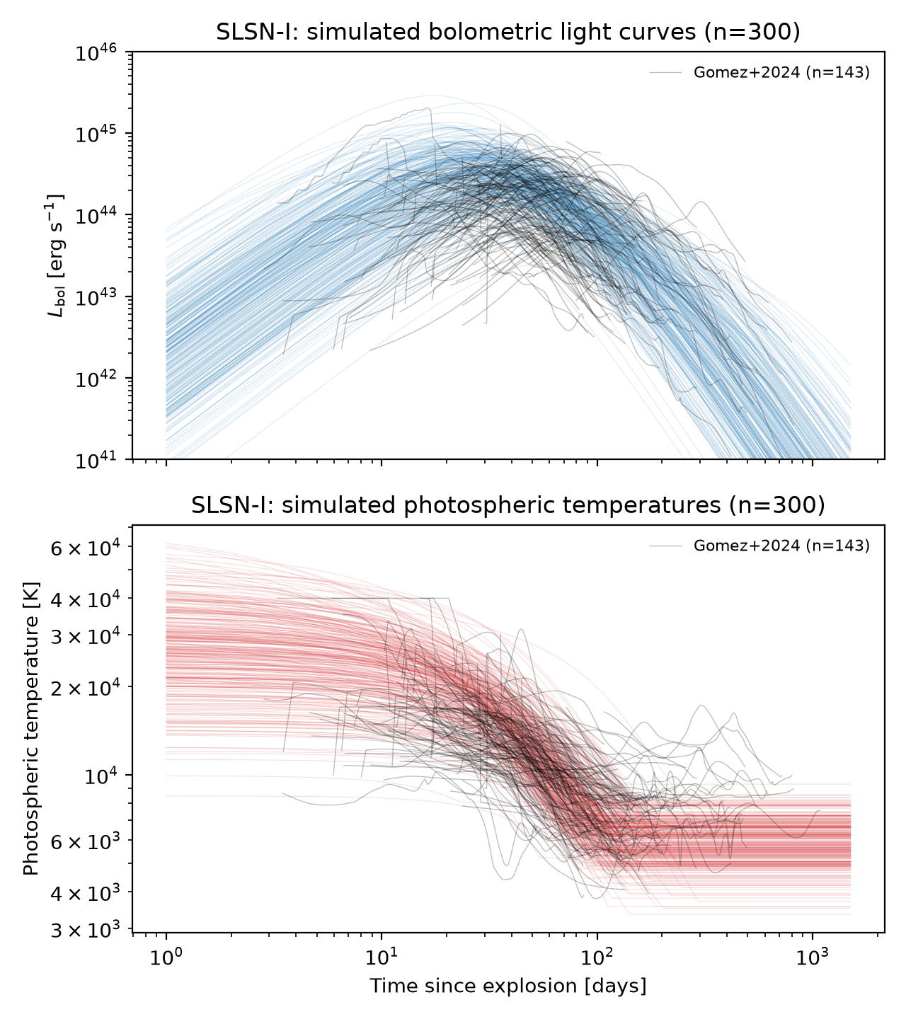
is the leakage parameter. We adopt the density-profile constant \(\beta=13.8\)[3]. The photosphere expands at the constant ejecta velocity \(v_\mathrm{ej}\), so its temperature follows the Stefan-Boltzmann law until it cools to a floor \(T_\mathrm{floor}\), after which it holds there (the photosphere then recedes rather than continuing to cool):

\[T(t) = \max\left\{\left[\frac{L(t)}{4\pi\sigma_\mathrm{SB}(v_\mathrm{ej}t)^2}\right]^{1/4},\ T_\mathrm{floor}\right\}, \qquad L_\nu(\nu, t) = L(t)\,\frac{\pi B_\nu(\nu, T(t))}{\sigma_\mathrm{SB}T(t)^4}.\]

Parameter	Symbol	Prior	Notes / Source
spin_period	\(P\)	TruncatedLogNormal(\(\log_{10}(P/\mathrm{ms})\); mean=:math:log_{10}(3.0), \(\sigma\)=0.104; bounds \([0.7, 20]\) ms)	Calibrated as a group with B_perp/M_ej (see note above); bounds are Nicholl et al.[4]’s own fit-prior range.
B_perp	\(B_\perp\)	TruncatedLogNormal(\(\log_{10}(B_\perp/10^{14}\,\mathrm{G})\); mean=:math:log_{10}(0.8), \(\sigma\)=0.192; bounds \([0.01, 10]\times10^{14}\) G)	Calibrated as a group with spin_period/M_ej (see note above); bounds are Nicholl et al.[4]’s own fit-prior range.
M_ej	\(M_\mathrm{ej}\)	TruncatedLogNormal(\(\log_{10}(M_\mathrm{ej}/M_\odot)\); mean=:math:log_{10}(4.8), \(\sigma\)=0.152; bounds \([0.1, 100]\,M_\odot\))	Calibrated as a group with spin_period/B_perp (see note above); bounds are Nicholl et al.[4]’s own fit-prior range.
v_ej	\(v_\mathrm{ej}\)	TruncatedNormal(\(v_\mathrm{ej}/10^4\,\mathrm{km\,s^{-1}}\); mean=0.9, \(\sigma\)=0.3; bounds \([0.1, 3.0]\))	\(\approx9000\ \mathrm{km\,s^{-1}}\), from \(\sqrt{2E_K/M_\mathrm{ej}}\) at the posterior median \(E_K=3.9\times10^{51}\) erg, \(M_\mathrm{ej}=4.8\,M_\odot\) [4]; width chosen here.
M_ns	\(M_\mathrm{NS}\)	Uniform(1.4, 2.2) \(M_\odot\)	Fit-prior range [4].
kappa	\(\kappa\)	Uniform(0.05, 0.2) \(\mathrm{cm^2\,g^{-1}}\)	Fit-prior range [4].
kappa_gamma	\(\kappa_\gamma\)	LogUniform(0.01, 1) \(\mathrm{cm^2\,g^{-1}}\)	Narrower than the fit-prior’s full \(0.01\)-\(100\ \mathrm{cm^2\,g^{-1}}\) range: only a few events have late enough data to constrain \(\kappa_\gamma\), but those that do favour similarly low values (e.g. SN 2015bn, \(\kappa_\gamma\approx0.01\)) [4].
T_floor	\(T_\mathrm{floor}\)	TruncatedNormal(6000 K, \(\sigma\)=1000 K; bounds \([3000, 10000]\) K)	Matches the fit prior exactly [4].

Simulated Light Curves

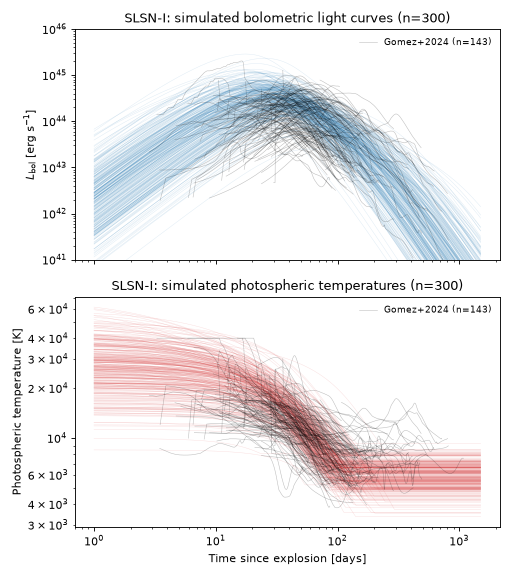
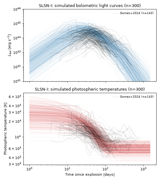
The plot below draws 300 random parameter realizations from the priors above and shows the resulting bolometric light curves and photospheric temperatures. Overlaid lightcurves are from Gomez et al.[9], which provides a curated set of SLSN-I light curves from the literature, with bolometric luminosities derived from multi-band photometry.

(Source code, png, hires.png, pdf)

---

Observability Summary

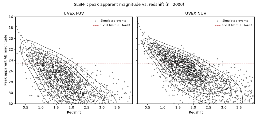
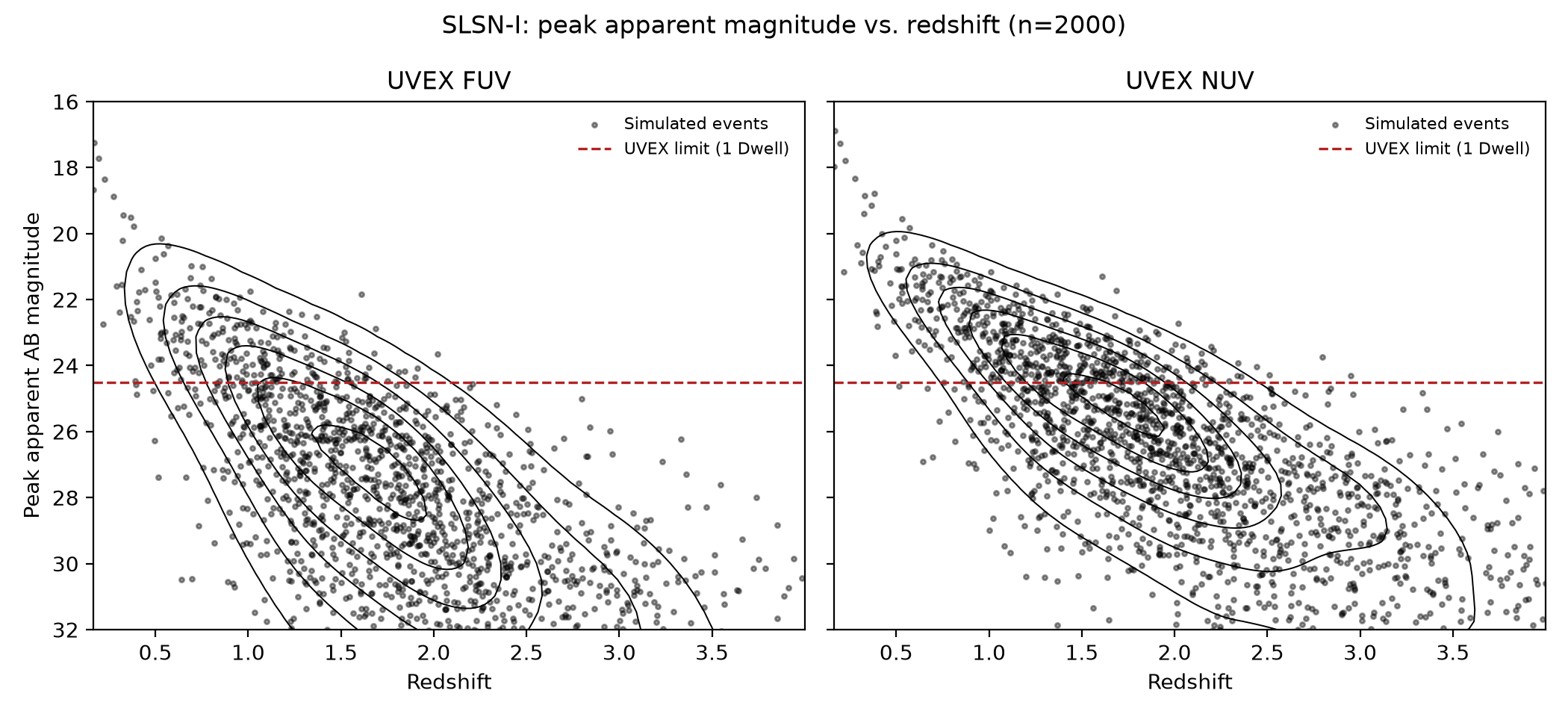
The light curve here has no single parameter that is exactly the bolometric peak time (\(L(t)\) is a numerically integrated diffusion solution), so each event’s peak apparent magnitude is found by searching a rest-frame time grid rather than evaluating at one closed-form epoch. Below are the redshifts \(z\) and corresponding bandpass peak apparent AB magnitudes \(m_\mathrm{AB}\) of 2000 simulated events drawn from the priors above, with the UVEX 1 Dwell limit of \(m<24.5\) overplotted. This justifies the \(z=4\) redshift limit adopted above.

(Source code, png, hires.png, pdf)

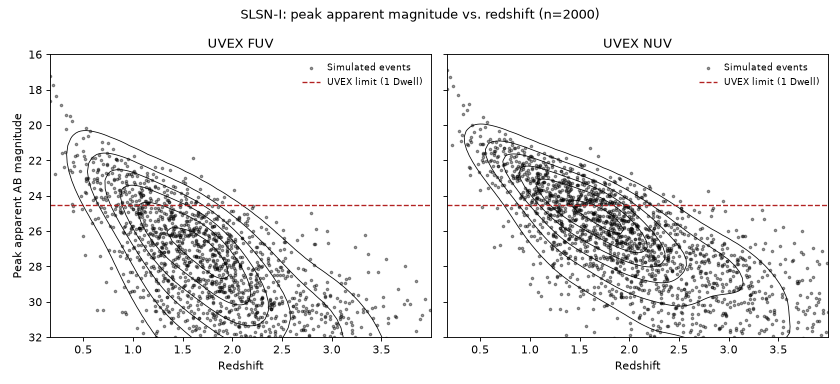
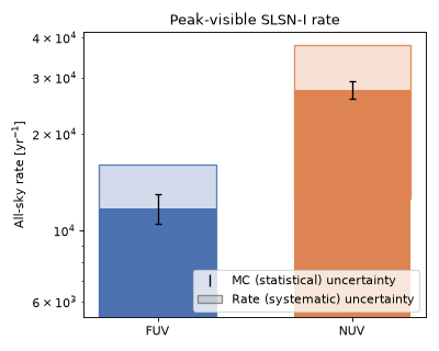
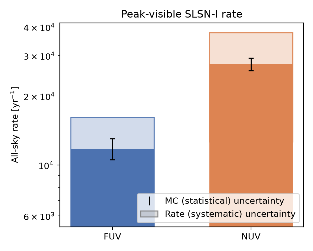
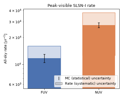
The anticipated rate of SLSNe-I detectable by UVEX at this limit is as follows, assuming that any event above the \(m<24.5\) limit is detectable, and that the population is isotropic and homogeneous in comoving volume out to \(z=4\):

(Source code, png, hires.png, pdf)

References

[1]

Daniel Kasen and Lars Bildsten. Supernova Light Curves Powered by Young Magnetars. \apj , 717(1):245–249, July 2010. arXiv:0911.0680, doi:10.1088/0004-637X/717/1/245.

[2]

S. E. Woosley. Bright Supernovae from Magnetar Birth. \apjl , 719(2):L204–L207, August 2010. arXiv:0911.0698, doi:10.1088/2041-8205/719/2/L204.

[3] (1,2)

W. D. Arnett. Type I supernovae. I - Analytic solutions for the early part of the light curve. \apj , 253:785–797, February 1982. doi:10.1086/159681.

[4] (1,2,3,4,5,6,7,8,9,10,11)

Matt Nicholl, James Guillochon, and Edo Berger. The Magnetar Model for Type I Superluminous Supernovae. I. Bayesian Analysis of the Full Multicolor Light-curve Sample with MOSFiT. \apj , 850(1):55, November 2017. arXiv:1706.00825, doi:10.3847/1538-4357/aa9334.

[5]

S. Q. Wang, L. J. Wang, Z. G. Dai, and X. F. Wu. Superluminous Supernovae Powered by Magnetars: Late-time Light Curves and Hard Emission Leakage. \apj , 799(1):107, January 2015. arXiv:1411.5126, doi:10.1088/0004-637X/799/1/107.

[6] (1,2)

Louis-Gregory Strolger, Tomas Dahlen, Steven A. Rodney, Or Graur, Adam G. Riess, Curtis McCully, Swara Ravindranath, Bahram Mobasher, and A. Kristin Shahady. The rate of core collapse supernovae to redshift 2.5 from the CANDELS and CLASH supernova surveys. The Astrophysical Journal, 813(2):93, 2015. arXiv:1509.06574, doi:10.1088/0004-637X/813/2/93.

[7]

Piero Madau and Mark Dickinson. Cosmic star-formation history. Annual Review of Astronomy and Astrophysics, 52:415–486, 2014. arXiv:1403.0007, doi:10.1146/annurev-astro-081811-125615.

[8] (1,2)

C. Frohmaier, C. R. Angus, M. Vincenzi, M. Sullivan, M. Smith, P. E. Nugent, S. B. Cenko, A. Gal-Yam, S. R. Kulkarni, N. M. Law, and R. M. Quimby. From core collapse to superluminous: the rates of massive stellar explosions from the Palomar Transient Factory. \mnras , 500(4):5142–5161, January 2021. arXiv:2010.15270, doi:10.1093/mnras/staa3607.

[9]

Sebastian Gomez, Matt Nicholl, Edo Berger, Peter K. Blanchard, V. Ashley Villar, and others. The Type I superluminous supernova catalogue - I. Light-curve properties, models, and catalogue description. \mnras , 535(1):471–515, November 2024. arXiv:2407.07946, doi:10.1093/mnras/stae2270.