Writing a Custom Model#

The previous page covered everything you do with a model: create one, evaluate it, sample from it. This page covers how to build one. If uvex_transients.models does not already have the physics you need, whether that is a new light curve shape, a new spectral shape, or an entirely new kind of photosphere, this is how you add it.

Every model in the package, no matter how complicated, comes down to the same two pieces: a function of some physical inputs, and a named set of parameters that function depends on. The base classes described in Models (and in the uvex_transients.models.core.base module docstring) handle everything around that function: parameter storage, sampling, unit conversion, the _log_cgs/_log/_cgs/plain method family, bolometric integration, redshifting, magnitudes. You supply the function itself, as a single method named _eval.

We will build a small toy transient over the course of this page: a light curve with a linear rise and an exponential decay, an exponentially cut off power-law spectrum, and the composite SED that comes from putting the two together. None of it is meant to describe a real astrophysical source. It exists so every step can be checked against a plot as we go.

Choosing What to Subclass#

There are four base classes to choose from, and the right one depends on what your model actually depends on.

Base class	Depends on	Use it when
`Lightcurve`	\(t\) only	You are describing how the total (frequency-integrated) brightness evolves with time, with no opinion about color.
`Spectrum`	\(\nu\) only	You are describing the shape of the spectrum at a single instant, with no opinion about how bright the source is or how that shape changes over time.
`ComposedSpectralModel`	a `Lightcurve` and a `Spectrum`, multiplied	Your source has a fixed spectral shape that just gets scaled up and down in brightness as it evolves. This covers most physically motivated SEDs and is the one you should reach for first.
`SpectralModel`	\(\nu\) and \(t\) jointly	The spectral shape itself changes over time, so it cannot be factored into an independent brightness curve and an independent color. A cooling blackbody, where the temperature (and therefore the whole shape of the spectrum) evolves with \(t\), is the running example of this in the package: `KilonovaCoolingBlackbodySED`.

Most of this page builds a Lightcurve and a Spectrum and composes them. The last worked example shows what it looks like to subclass SpectralModel directly, for the cases where composition is not enough.

The One Method You Have to Write: `_eval`#

Whichever base class you subclass, the contract for _eval is the same in spirit:

It is a classmethod, not an instance method. Every quantity a model produces is a pure function of the parameter values you pass it, so no model instance is needed to evaluate it (only to store a particular configuration of parameters for later sampling).
Its inputs and output are unit-stripped, plain numpy.ndarray objects, always in cgs units (seconds, Hz, erg/s, Kelvin, and so on).
It returns a natural log, not the quantity itself.
Inputs combine by ordinary NumPy broadcasting. Nothing inserts a “batch” or “sample” axis for you; if you want to evaluate several parameter realizations against a shared time or frequency grid, you reshape the arrays yourself, exactly as the overview page’s population example does with a trailing [:, None].

Working in log space is not a stylistic choice. Bolometric luminosities span tens of orders of magnitude across a population, and many of the shapes in this package (power laws, blackbodies, exponential tails) are most naturally written as sums of logs rather than products of very large or very small numbers. Every public method built on top of _eval (eval, eval_cgs, mag, and the rest) handles converting back to linear space, attaching units, and validating inputs, so _eval itself can stay a short, exact expression.

Declaring Parameters#

A model’s parameters are declared once, as a class-level dict of Parameter objects:

from astropy import units as u
from uvex_transients.models.core import Parameter, LogNormalPrior

_DEFAULT_PARAMETERS = {
    "amplitude": Parameter(
        prior=LogNormalPrior(mean=0.0, sigma=0.5),
        scale=1e43 * u.erg / u.s,
        description="Peak bolometric luminosity.",
        latex=r"A",
    ),
}

Three fields matter most:

prior: Where random draws come from. The built-ins in uvex_transients.models.core.priors cover the common cases: UniformPrior, NormalPrior, LogNormalPrior, TruncatedNormalPrior, ExponentialPrior, PowerLawPrior, ConstantPrior (for a parameter that should behave as fixed unless someone overrides it), and DiscretePrior.
scale: The characteristic physical size of the parameter, as a Quantity (or a bare number for a genuinely dimensionless parameter). Every physical value is divided by scale before the prior sees it, which is what lets prior itself be written in convenient, unit-free terms rather than needing to know about days versus seconds or erg/s versus solar luminosities.
transform: An optional reparameterization applied on top of scale, most often "log" or "log10". A strictly positive, many-orders-of-magnitude quantity (an amplitude, a temperature) samples much better from a Gaussian prior on its logarithm than from a Gaussian prior on the value itself; transform="log10" is exactly how amplitude and T0 are handled in KilonovaCoolingBlackbodySED.

description and latex are optional but worth filling in: the former shows up in __repr__() and generated docs, the latter in plot labels built from the model automatically.

Inside _eval, parameters arrive as plain keyword arguments, already unit-stripped and in cgs (so amplitude above arrives as a bare float in erg/s, not a Quantity). You can either accept them generically through **parameters and index into the dict, or narrow the signature to your model’s own named parameters, which is the pattern used throughout the package itself (see any of the _eval overrides in uvex_transients.models.lightcurves.generic) because it lets a type checker and your editor catch a misspelled parameter name.

A Custom Light Curve, From Scratch#

Suppose the flare shapes already in uvex_transients.models.lightcurves do not fit: we want a light curve that rises linearly from zero, peaks at t_peak, and then decays exponentially with timescale tau_decay.

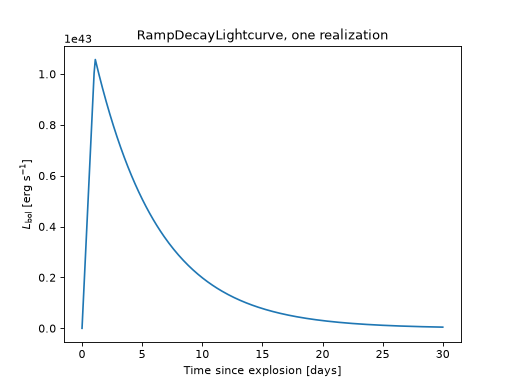
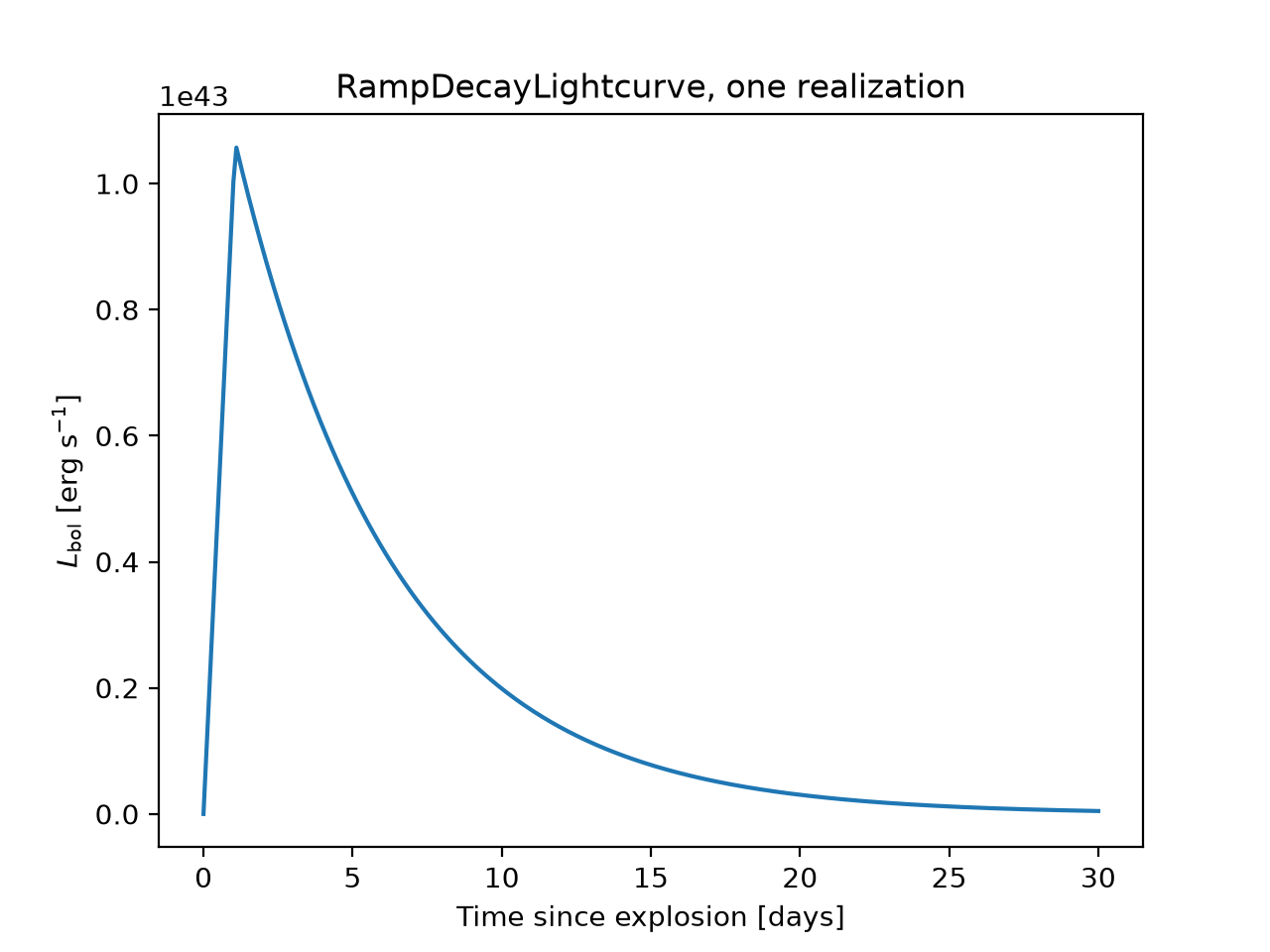
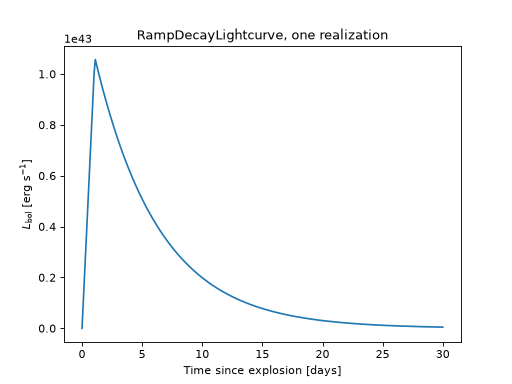
\[\begin{split}L(t) = \begin{cases} A\, (t / t_\mathrm{peak}), & 0 \le t \le t_\mathrm{peak} \\ A\, \exp\!\left(-\dfrac{t - t_\mathrm{peak}}{\tau_\mathrm{decay}}\right), & t > t_\mathrm{peak} \end{cases}\end{split}\]

Both branches agree at \(t = t_\mathrm{peak}\), where \(L = A\) exactly. Here is the whole class:

from typing import ClassVar

import numpy as np
from astropy import units as u

from uvex_transients.models.core import Lightcurve, LogNormalPrior, Parameter
from uvex_transients.models._typing import CGSParameterValue, FloatArray
from uvex_transients.models._utils import _BOL_LUM_UNIT


class RampDecayLightcurve(Lightcurve):
    r"""A linear rise to `t_peak`, followed by an exponential decay."""

    _DEFAULT_PARAMETERS: ClassVar[dict[str, Parameter]] = {
        "amplitude": Parameter(
            prior=LogNormalPrior(mean=0.0, sigma=0.5),
            scale=1e43 * _BOL_LUM_UNIT,
            description="Peak bolometric luminosity.",
            latex=r"A",
        ),
        "t_peak": Parameter(
            prior=LogNormalPrior(mean=0.0, sigma=0.5),
            scale=1.0 * u.day,
            description="Time of peak luminosity since explosion.",
            latex=r"t_\mathrm{peak}",
        ),
        "tau_decay": Parameter(
            prior=LogNormalPrior(mean=0.0, sigma=0.5),
            scale=5.0 * u.day,
            description="Exponential decay timescale past t_peak.",
            latex=r"\tau_\mathrm{decay}",
        ),
    }

    @classmethod
    def _eval(cls, t: FloatArray, **parameters: CGSParameterValue) -> FloatArray:
        amplitude = parameters["amplitude"]
        t_peak = parameters["t_peak"]
        tau_decay = parameters["tau_decay"]

        # `t_peak` is strictly positive by its prior's support, so `t = 0`
        # always falls on the rising branch: log(0 / t_peak) = -inf is the
        # correct limit there, not an error.
        with np.errstate(divide="ignore"):
            log_rise = np.log(t / t_peak)

        log_decay = -(t - t_peak) / tau_decay

        return np.log(amplitude) + np.where(t <= t_peak, log_rise, log_decay)

A few things worth pointing out about this class, because they generalize to every model you write:

_eval never touches units. t, amplitude, t_peak, and tau_decay are all plain floats in seconds or erg/s by the time they reach it; the base class handled the conversion in eval_log().
The branch that is discarded at each t is allowed to be numerically ugly (here, a divide warning at t = 0), as long as it is masked out by numpy.where() before it reaches the caller. Suppressing the warning explicitly, with a comment explaining why it is expected, is the convention used everywhere else in the package.
There is no __init__ to write. Parameter storage, copying, the Mapping interface, and sampling all come from _ModelBase.

Once defined, it behaves exactly like any built-in light curve:

import numpy as np
import matplotlib.pyplot as plt
from astropy import units as u

from uvex_transients.models.core import Lightcurve, LogNormalPrior, Parameter
from uvex_transients.models._typing import CGSParameterValue, FloatArray
from uvex_transients.models._utils import _BOL_LUM_UNIT


class RampDecayLightcurve(Lightcurve):
    _DEFAULT_PARAMETERS = {
        "amplitude": Parameter(
            prior=LogNormalPrior(mean=0.0, sigma=0.5), scale=1e43 * _BOL_LUM_UNIT,
        ),
        "t_peak": Parameter(prior=LogNormalPrior(mean=0.0, sigma=0.5), scale=1.0 * u.day),
        "tau_decay": Parameter(prior=LogNormalPrior(mean=0.0, sigma=0.5), scale=5.0 * u.day),
    }

    @classmethod
    def _eval(cls, t: FloatArray, **parameters: CGSParameterValue) -> FloatArray:
        amplitude, t_peak, tau_decay = (
            parameters["amplitude"], parameters["t_peak"], parameters["tau_decay"],
        )
        with np.errstate(divide="ignore"):
            log_rise = np.log(t / t_peak)
        log_decay = -(t - t_peak) / tau_decay
        return np.log(amplitude) + np.where(t <= t_peak, log_rise, log_decay)

lc = RampDecayLightcurve()
params = lc.sample_parameters(rng=0)

t = np.linspace(0, 30, 300) * u.day
L_bol = lc.eval(t, **params)

plt.plot(t.to_value(u.day), L_bol.to_value(u.erg / u.s))
plt.xlabel("Time since explosion [days]")
plt.ylabel(r"$L_\mathrm{bol}$ [erg s$^{-1}$]")
plt.title("RampDecayLightcurve, one realization")

(Source code, png, hires.png, pdf)

A Custom Spectral Shape, From Scratch#

A Spectrum follows the same pattern as a Lightcurve, but over frequency instead of time, and with one extra piece: because \(S(\nu)\) need not integrate to any particular value by construction, eval_normalization() has to know what \(\int S(\nu)\,d\nu\) actually is. By default it finds that out the expensive way, by numerically integrating your _eval over the frequency range given by the class’s _DOMAIN attribute. If your shape has a closed-form integral, override _eval_normalization() yourself, both for speed and to avoid any quadrature error; BlackbodySpectrum and PowerLawSpectrum both do this. If it does not, the default is there to fall back on, and correctness costs you nothing beyond evaluation speed.

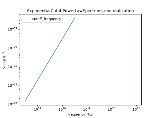
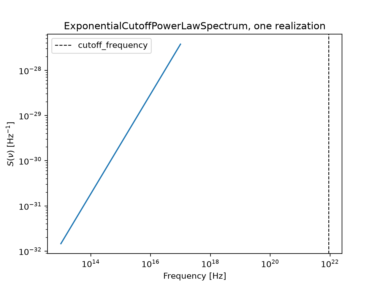
Here we build a power law with an exponential cutoff, a common shape for the high-frequency tail of a nonthermal spectrum, and lean on the numerical default rather than deriving a closed form:

from typing import ClassVar

import numpy as np
from astropy import units as u

from uvex_transients.models.core import NormalPrior, LogNormalPrior, Parameter, Spectrum
from uvex_transients.models._typing import CGSParameterValue, FloatArray


class ExponentialCutoffPowerLawSpectrum(Spectrum):
    r"""A power law that turns over exponentially above `cutoff_frequency`."""

    _DEFAULT_PARAMETERS: ClassVar[dict[str, Parameter]] = {
        "spectral_index": Parameter(
            prior=NormalPrior(mean=1.0, sigma=0.3),
            scale=1.0,
            description="Frequency-space power-law index below the cutoff.",
            latex=r"\alpha",
        ),
        "cutoff_frequency": Parameter(
            prior=LogNormalPrior(mean=0.0, sigma=0.3),
            scale=1e15 * u.Hz,
            description="Frequency above which the spectrum turns over exponentially.",
            latex=r"\nu_\mathrm{cut}",
        ),
    }

    @classmethod
    def _eval(  # type: ignore[override]
        cls, nu: FloatArray, *, spectral_index: CGSParameterValue, cutoff_frequency: CGSParameterValue
    ) -> FloatArray:
        x = nu / cutoff_frequency

        with np.errstate(divide="ignore"):
            log_shape = spectral_index * np.log(x) - x

        return log_shape - np.log(cutoff_frequency)

We keep spectral_index centered above \(-1\), so the shape stays integrable as \(\nu \to 0\); the exponential factor already takes care of the high-frequency end. _eval_normalization is left untouched, so it falls back to numerical quadrature over the default domain, (0, inf) Hz, the first time it is needed:

import numpy as np
import matplotlib.pyplot as plt
from astropy import units as u

from uvex_transients.models.core import NormalPrior, LogNormalPrior, Parameter, Spectrum
from uvex_transients.models._typing import CGSParameterValue, FloatArray


class ExponentialCutoffPowerLawSpectrum(Spectrum):
    _DEFAULT_PARAMETERS = {
        "spectral_index": Parameter(prior=NormalPrior(mean=1.0, sigma=0.3), scale=1.0),
        "cutoff_frequency": Parameter(
            prior=LogNormalPrior(mean=0.0, sigma=0.3), scale=1e15 * u.Hz,
        ),
    }

    @classmethod
    def _eval(cls, nu: FloatArray, *, spectral_index, cutoff_frequency) -> FloatArray:
        x = nu / cutoff_frequency
        with np.errstate(divide="ignore"):
            log_shape = spectral_index * np.log(x) - x
        return log_shape - np.log(cutoff_frequency)

spec = ExponentialCutoffPowerLawSpectrum()
spec["cutoff_frequency"].fix(3000 * u.AA.to(u.Hz, equivalencies=u.spectral()) * u.Hz)
params = spec.sample_parameters(rng=1)

nu = np.geomspace(1e13, 1e17, 300) * u.Hz
S = spec.eval(nu, **params)

plt.plot(nu.to_value(u.Hz), S.to_value(1 / u.Hz))
plt.xscale("log")
plt.yscale("log")
plt.xlabel(r"Frequency [Hz]")
plt.ylabel(r"$S(\nu)$ [Hz$^{-1}$]")
plt.title("ExponentialCutoffPowerLawSpectrum, one realization")
plt.axvline(
    spec["cutoff_frequency"].fixed_value.value, color="k", ls="--", lw=1, label="cutoff_frequency",
)
plt.legend()

(Source code, png, hires.png, pdf)

Combining Them Into a Full SED#

With a Lightcurve and a Spectrum in hand, building the full \(L_\nu(\nu, t)\) model is just naming the two component classes:

from typing import ClassVar

from uvex_transients.models.core import ComposedSpectralModel


class ToyFlareSED(ComposedSpectralModel):
    _LIGHTCURVE_CLASS: ClassVar = RampDecayLightcurve
    _SPECTRUM_CLASS: ClassVar = ExponentialCutoffPowerLawSpectrum

No _eval to write this time. At class-definition time, __init_subclass__() merges the two components’ _DEFAULT_PARAMETERS dicts into one flat namespace (checking that no parameter name is shared between them), and every method your model needs, _eval(), _eval_bolometric(), and _eval_spectrum(), is built out of exact, closed-form combinations of the light curve’s and spectrum’s own primitives. None of the numerical-quadrature fallbacks on SpectralModel itself are ever reached for a composed model.

From here, ToyFlareSED behaves exactly like KilonovaCoolingBlackbodySED did on the overview page: sample parameters, evaluate, plot a population.

import numpy as np
import matplotlib.pyplot as plt
from astropy import units as u

from uvex_transients.models.core import (
    ComposedSpectralModel, Lightcurve, LogNormalPrior, NormalPrior, Parameter, Spectrum,
)
from uvex_transients.models._typing import CGSParameterValue, FloatArray
from uvex_transients.models._utils import _BOL_LUM_UNIT


class RampDecayLightcurve(Lightcurve):
    _DEFAULT_PARAMETERS = {
        "amplitude": Parameter(
            prior=LogNormalPrior(mean=0.0, sigma=0.5), scale=1e43 * _BOL_LUM_UNIT,
        ),
        "t_peak": Parameter(prior=LogNormalPrior(mean=0.0, sigma=0.5), scale=1.0 * u.day),
        "tau_decay": Parameter(prior=LogNormalPrior(mean=0.0, sigma=0.5), scale=5.0 * u.day),
    }

    @classmethod
    def _eval(cls, t: FloatArray, **parameters: CGSParameterValue) -> FloatArray:
        amplitude, t_peak, tau_decay = (
            parameters["amplitude"], parameters["t_peak"], parameters["tau_decay"],
        )
        with np.errstate(divide="ignore"):
            log_rise = np.log(t / t_peak)
        log_decay = -(t - t_peak) / tau_decay
        return np.log(amplitude) + np.where(t <= t_peak, log_rise, log_decay)


class ExponentialCutoffPowerLawSpectrum(Spectrum):
    _DEFAULT_PARAMETERS = {
        "spectral_index": Parameter(prior=NormalPrior(mean=1.0, sigma=0.3), scale=1.0),
        "cutoff_frequency": Parameter(
            prior=LogNormalPrior(mean=0.0, sigma=0.3), scale=1e15 * u.Hz,
        ),
    }

    @classmethod
    def _eval(cls, nu: FloatArray, *, spectral_index, cutoff_frequency) -> FloatArray:
        x = nu / cutoff_frequency
        with np.errstate(divide="ignore"):
            log_shape = spectral_index * np.log(x) - x
        return log_shape - np.log(cutoff_frequency)


class ToyFlareSED(ComposedSpectralModel):
    _LIGHTCURVE_CLASS = RampDecayLightcurve
    _SPECTRUM_CLASS = ExponentialCutoffPowerLawSpectrum

rng = np.random.default_rng(20260911)
n_samples = 200

params = ToyFlareSED().sample_parameters(size=n_samples, rng=rng)
params_grid = {name: value[:, None] for name, value in params.items()}

t = np.linspace(0, 30, 200) * u.day
L_bol = ToyFlareSED.eval_bolometric(t, **params_grid)

plt.plot(t.to_value(u.day), L_bol.to_value(u.erg / u.s).T, color="C0", lw=0.5, alpha=0.15)
plt.yscale("log")
plt.xlabel("Time since explosion [days]")
plt.ylabel(r"$L_\mathrm{bol}$ [erg s$^{-1}$]")
plt.title(f"{n_samples} simulated ToyFlareSED light curves")

(Source code, png, hires.png, pdf)

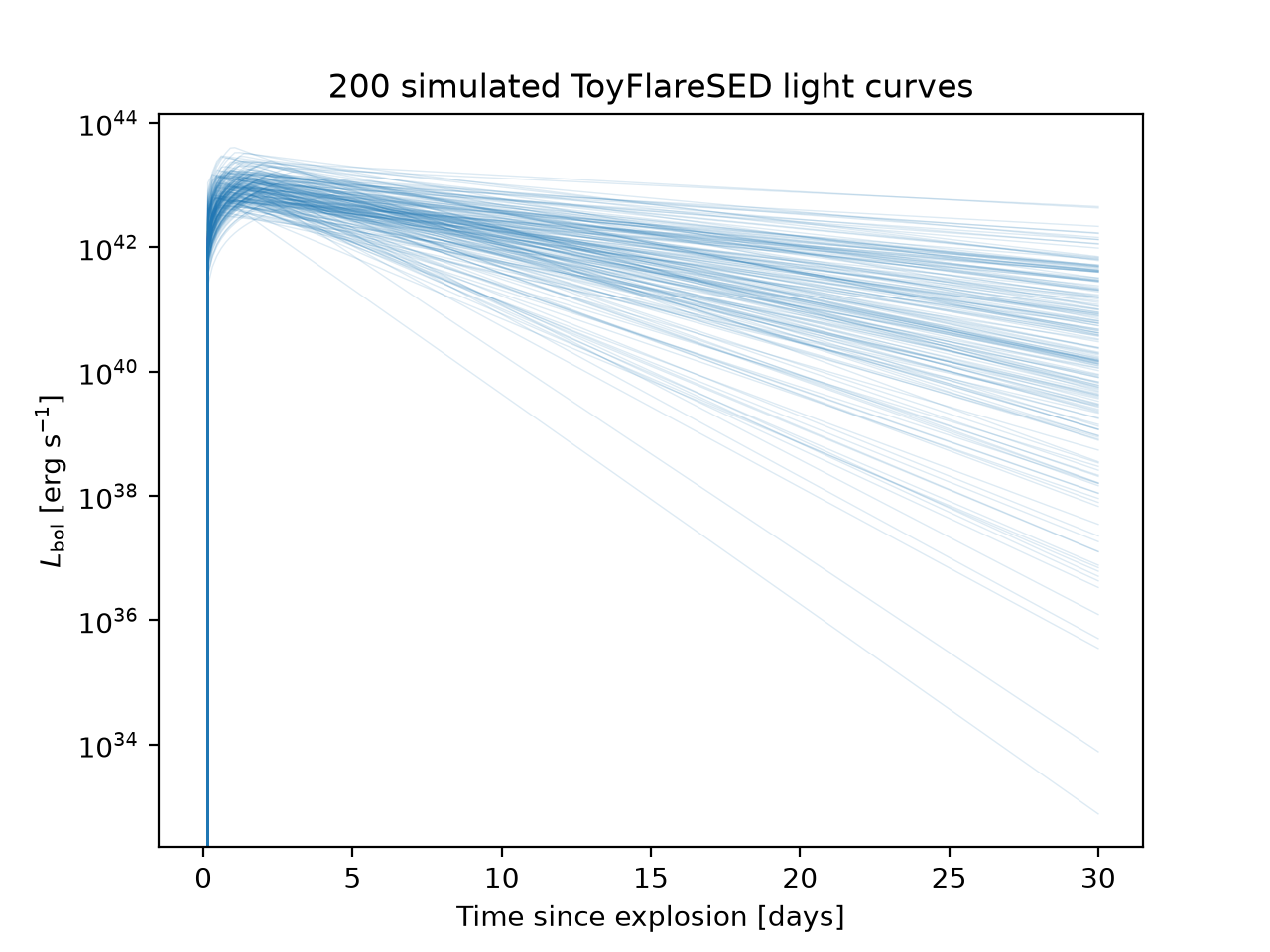
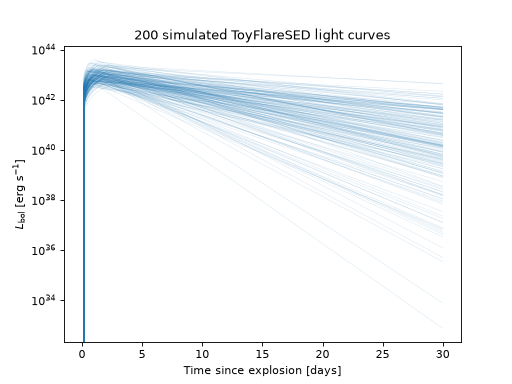
Because sample_parameters draws from the merged parameter set, a single call already covers both the light curve and the spectral shape: amplitude, t_peak, and tau_decay came from RampDecayLightcurve, spectral_index and cutoff_frequency from ExponentialCutoffPowerLawSpectrum, and neither component needed to know the other existed.

When a Light Curve and a Spectrum Are Not Enough#

Composition assumes the spectral shape is fixed and only the overall brightness changes with time. That breaks down as soon as color itself evolves, most commonly because a photospheric temperature is cooling. For that case, subclass SpectralModel directly and implement _eval(nu, t, **parameters) yourself.

You do not have to start from nothing even here. KilonovaCoolingBlackbodySED is built almost entirely out of the same Lightcurve/Spectrum primitives used above, just wired together by hand instead of through ComposedSpectralModel:

Its bolometric evolution is a GaussianRiseBrokenPowerLawLightcurve, so _eval_bolometric simply calls that class’s own _eval and is exact, with no integration needed.
Its spectral shape at any instant is a BlackbodySpectrum, but evaluated at a temperature that is itself a function of t, so _eval_spectrum computes T(t) first and then calls BlackbodySpectrum._eval at that temperature.
_eval itself is just the sum of the two logs: \(\log L_\nu(\nu, t) = \log L_\mathrm{bol}(t) + \log S(\nu, T(t))\).

The pattern generalizes: reuse existing Lightcurve/Spectrum classes as building blocks wherever you can, even when the base class you are subclassing directly is SpectralModel itself. Writing everything from bare NumPy is rarely necessary.

Testing a New Model#

New models are not given bespoke tests. tests.models._contracts defines shared, inheritable pytest contracts, LightcurveContract, SpectrumContract, and SpectralModelContract, covering instantiation, the parameter-override behavior every model shares, and the eval*-family consistency checks described earlier on this page (verified against independent numerical integration). Covering a new model means adding a two-line class to the matching test module:

# tests/models/test_seds.py
from mypackage.models import ToyFlareSED
from ._contracts import SpectralModelContract


class TestToyFlareSED(SpectralModelContract):
    model_class = ToyFlareSED

RampDecayLightcurve and ExponentialCutoffPowerLawSpectrum would get their own two-line classes in tests/models/test_lightcurves.py and tests/models/test_spectra.py, respectively, inheriting LightcurveContract and SpectrumContract. Each test module ends with a completeness check that walks every concrete subclass of the relevant base class and fails loudly if one of them has no matching Test* class, so a new model added without a corresponding test line cannot pass silently.

Next Steps#

A model on its own is only an SED. To simulate a population of sources with it, that is, to give it a sky distribution, a volumetric rate, and a redshift range, pair it with a TransientBase subclass, covered in Transients and, for the pairing step specifically, in Writing a Custom Transient.

Writing a Custom Model#

Choosing What to Subclass#

The One Method You Have to Write: _eval#

Declaring Parameters#

A Custom Light Curve, From Scratch#

A Custom Spectral Shape, From Scratch#

Combining Them Into a Full SED#

When a Light Curve and a Spectrum Are Not Enough#

Testing a New Model#

Next Steps#

The One Method You Have to Write: `_eval`#