TDE End-to-End Simulation

A minimal example of an end-to-end simulation of transient yields from a UVEX survey schedule. In this example, we’ll determine the anticipated yield of TDEs with the default UVEX schedule. To do this, we’ll take the following steps:

1. Configure our transient class, including changing any relevant priors, durations, etc.

2. Draw events from the schedule, and then

3. Filter events by observability.

4. Generate synthetic photometry.

Load the schedule and set up the population

We can start by loading the default schedule using get_schedule(). We’ll also want to get the TDE class configured and load the simulator.

Note

At this stage, you can make modifications to priors as needed.

import numpy as np
from astropy import units as u
from m4opt.missions import uvex
from matplotlib import pyplot as plt

from uvex_transients.simulation.core import SurveySimulator
from uvex_transients.surveys import get_schedule
from uvex_transients.transients.TDEs import TidalDisruptionEvent
from uvex_transients.utils.plotting import (
    add_funnel_legend,
    compute_funnel_bounds,
    get_band_color,
    plot_band_light_curve,
    plot_detection_funnel,
    resolve_fig_axes,
    set_plot_style,
)

set_plot_style()

schedule = get_schedule()
tde = TidalDisruptionEvent()
simulator = SurveySimulator(schedule, transients={"tde": tde}, simulation_seed=42)

Sample a Monte Carlo population

We now want to draw synthetic events for the schedule. This uses a windowed sampling technique so that only events which fall within the instrument’s footprint at some point during their duration are sampled.

Note

For events with very high intrinsic rates, it can be useful to provide a downsample value to reduce the number of simulated events. This can then be used to rescale to the total number of events at a later point in the analysis.

TIME_BINS = 20
NSIDE = 64
DOWNSAMPLE = 20

catalog = simulator.generate_events(time_bins=TIME_BINS, nside=NSIDE, downsample=DOWNSAMPLE)
print(f"Sampled {len(catalog) * DOWNSAMPLE} TDEs across {TIME_BINS} time bin(s) at NSIDE={NSIDE}.")

Generating events:   0%|          | 0/20 [00:00<?, ?bin/s]
Generating events:   0%|          | 0/20 [00:00<?, ?bin/s, bin=1/20, type=tde]
Generating events:   5%|▌         | 1/20 [00:06<02:08,  6.77s/bin, bin=1/20, type=tde]
Generating events:   5%|▌         | 1/20 [00:06<02:08,  6.77s/bin, bin=2/20, type=tde]
Generating events:  10%|█         | 2/20 [00:06<02:01,  6.77s/bin, bin=3/20, type=tde]
Generating events:  15%|█▌        | 3/20 [00:06<00:30,  1.82s/bin, bin=3/20, type=tde]
Generating events:  15%|█▌        | 3/20 [00:06<00:30,  1.82s/bin, bin=4/20, type=tde]
Generating events:  20%|██        | 4/20 [00:07<00:29,  1.82s/bin, bin=5/20, type=tde]
Generating events:  25%|██▌       | 5/20 [00:07<00:13,  1.07bin/s, bin=5/20, type=tde]
Generating events:  25%|██▌       | 5/20 [00:07<00:13,  1.07bin/s, bin=6/20, type=tde]
Generating events:  30%|███       | 6/20 [00:07<00:13,  1.07bin/s, bin=7/20, type=tde]
Generating events:  35%|███▌      | 7/20 [00:07<00:07,  1.74bin/s, bin=7/20, type=tde]
Generating events:  35%|███▌      | 7/20 [00:07<00:07,  1.74bin/s, bin=8/20, type=tde]
Generating events:  40%|████      | 8/20 [00:07<00:06,  1.74bin/s, bin=9/20, type=tde]
Generating events:  45%|████▌     | 9/20 [00:07<00:04,  2.55bin/s, bin=9/20, type=tde]
Generating events:  45%|████▌     | 9/20 [00:07<00:04,  2.55bin/s, bin=10/20, type=tde]
Generating events:  50%|█████     | 10/20 [00:07<00:03,  2.55bin/s, bin=11/20, type=tde]
Generating events:  55%|█████▌    | 11/20 [00:07<00:02,  3.50bin/s, bin=11/20, type=tde]
Generating events:  55%|█████▌    | 11/20 [00:07<00:02,  3.50bin/s, bin=12/20, type=tde]
Generating events:  60%|██████    | 12/20 [00:07<00:02,  3.50bin/s, bin=13/20, type=tde]
Generating events:  65%|██████▌   | 13/20 [00:07<00:01,  4.54bin/s, bin=13/20, type=tde]
Generating events:  65%|██████▌   | 13/20 [00:07<00:01,  4.54bin/s, bin=14/20, type=tde]
Generating events:  70%|███████   | 14/20 [00:07<00:01,  4.54bin/s, bin=15/20, type=tde]
Generating events:  75%|███████▌  | 15/20 [00:08<00:00,  5.44bin/s, bin=15/20, type=tde]
Generating events:  75%|███████▌  | 15/20 [00:08<00:00,  5.44bin/s, bin=16/20, type=tde]
Generating events:  80%|████████  | 16/20 [00:08<00:00,  5.44bin/s, bin=17/20, type=tde]
Generating events:  85%|████████▌ | 17/20 [00:08<00:00,  6.70bin/s, bin=17/20, type=tde]
Generating events:  85%|████████▌ | 17/20 [00:08<00:00,  6.70bin/s, bin=18/20, type=tde]
Generating events:  90%|█████████ | 18/20 [00:08<00:00,  6.70bin/s, bin=19/20, type=tde]
Generating events:  95%|█████████▌| 19/20 [00:08<00:00,  8.24bin/s, bin=19/20, type=tde]
Generating events:  95%|█████████▌| 19/20 [00:08<00:00,  8.24bin/s, bin=20/20, type=tde]
Generating events: 100%|██████████| 20/20 [00:08<00:00,  2.39bin/s, bin=20/20, type=tde]
Sampled 115360 TDEs across 20 time bin(s) at NSIDE=64.

Screen the population

Two progressively more expensive passes narrow the freshly-sampled catalog down to the events that matter.

1. filter_by_limiting_magnitude() asks whether an event could ever clear a fixed magnitude limit.

2. filter_by_snr() asks the real question: is the event ever detected above a given SNR at an observation the schedule actually made?

MAG_LIMIT = 25.0
SNR_THRESHOLD = 5.0

mag_filtered = simulator.filter_by_limiting_magnitude(catalog, uvex, mag_limit=MAG_LIMIT)
print(f"{len(mag_filtered) * DOWNSAMPLE} could ever clear {MAG_LIMIT} AB mag.")

detected = simulator.filter_by_snr(mag_filtered, uvex, snr_threshold=SNR_THRESHOLD)
print(f"{len(detected) * DOWNSAMPLE} were detected above SNR={SNR_THRESHOLD}.")

Filtering by mag limit:   0%|          | 0/2 [00:00<?, ?chunk/s]
Filtering by mag limit:   0%|          | 0/2 [00:00<?, ?chunk/s, chunk=1/2, type=tde]
Filtering by mag limit:  50%|█████     | 1/2 [00:00<00:00,  1.46chunk/s, chunk=1/2, type=tde]
Filtering by mag limit:  50%|█████     | 1/2 [00:00<00:00,  1.46chunk/s, chunk=2/2, type=tde]
Filtering by mag limit: 100%|██████████| 2/2 [00:00<00:00,  2.63chunk/s, chunk=2/2, type=tde]
27140 could ever clear 25.0 AB mag.

Filtering by SNR:   0%|          | 0/1 [00:00<?, ?chunk/s]
Filtering by SNR:   0%|          | 0/1 [00:00<?, ?chunk/s, chunk=1/1, type=tde]
Filtering by SNR: 100%|██████████| 1/1 [00:00<00:00,  1.06chunk/s, chunk=1/1, type=tde]
Filtering by SNR: 100%|██████████| 1/1 [00:00<00:00,  1.06chunk/s, chunk=1/1, type=tde]
13160 were detected above SNR=5.0.

Detection funnel

Each stage’s raw count carries two distinct sources of uncertainty: MC (statistical) uncertainty from having only finitely many simulated draws (a black Clopper-Pearson error bar), and rate (systematic) uncertainty from the literature normalization underlying TDE’s event rate itself (a pale shaded band, from RATE_CI). See compute_funnel_bounds() for how the two are computed.

stages = ["Sampled", f"Mag < {MAG_LIMIT}", f"SNR > {SNR_THRESHOLD}"]
raw_counts = [len(catalog), len(mag_filtered), len(detected)]
counts = [c * DOWNSAMPLE for c in raw_counts]

mc_lower, mc_upper, rate_lower, rate_upper = compute_funnel_bounds(raw_counts, rate_ci=tde.RATE_CI)

fig, ax = resolve_fig_axes()
plot_detection_funnel(
    ax,
    x=np.arange(len(stages)),
    counts=np.asarray(counts, dtype=float),
    mc_lower=mc_lower * DOWNSAMPLE,
    mc_upper=mc_upper * DOWNSAMPLE,
    rate_lower=rate_lower * DOWNSAMPLE,
    rate_upper=rate_upper * DOWNSAMPLE,
)
ax.set_xticks(np.arange(len(stages)), stages)
ax.set_yscale("log")
for i, count in enumerate(counts):
    ax.text(i, rate_upper[i] * DOWNSAMPLE, f"{count:,}", ha="center", va="bottom")
ax.set_ylabel("Number of TDEs")
ax.set_title("TDE detection funnel")
add_funnel_legend(ax)
fig.tight_layout()

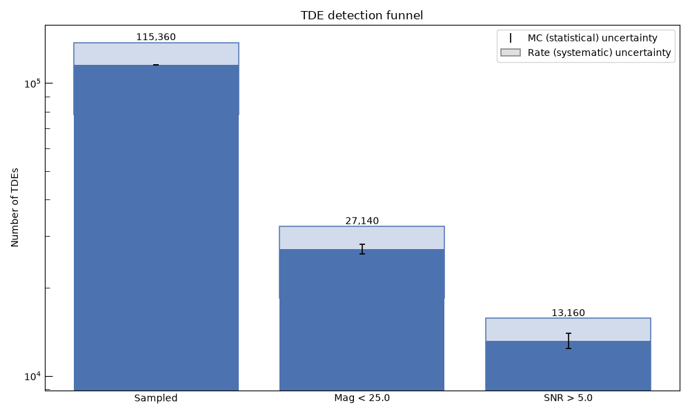
Black error bars are the MC (statistical) uncertainty on each stage’s count, from treating it as a binomial subsample of the raw simulated draws (Clopper-Pearson); the pale shaded band is the rate (systematic) uncertainty from the TDE rate’s own literature normalization (RATE_CI), which scales every stage by the same factor rather than shrinking as the sample is cut down.

Sky distribution

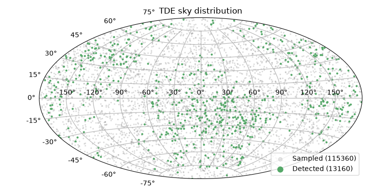
The sampled population traces the schedule’s own footprint; the detected subset is whatever fraction of it UVEX actually caught above \(\mathrm{SNR}=5\).

# sphinx_gallery_thumbnail_number = 2
fig, ax = resolve_fig_axes(fig_size=(8, 4), subplot_kw={"projection": "aitoff"})
ax.grid(True)

ra_sampled = catalog.coord.ra.wrap_at(180 * u.deg).radian
ra_detected = detected.coord.ra.wrap_at(180 * u.deg).radian

ax.scatter(
    ra_sampled,
    catalog.coord.dec.radian,
    s=2,
    alpha=0.2,
    color="#888888",
    label=f"Sampled ({DOWNSAMPLE * len(catalog)})",
)
ax.scatter(
    ra_detected, detected.coord.dec.radian, s=4, color="#55A868", label=f"Detected ({DOWNSAMPLE * (len(detected))})"
)
ax.legend(loc="lower right", markerscale=4)
ax.set_title("TDE sky distribution")
fig.tight_layout()

An example light curve

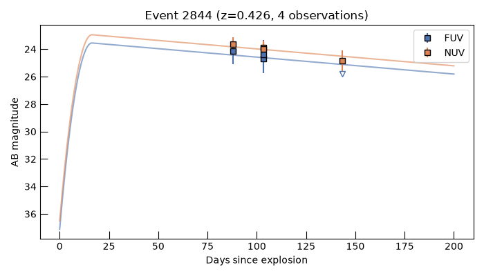
Reconstruct one detected event as a real Event (get_events()) and run full synthetic photometry (simulate_photometry()) against every observation the schedule actually made of it.

rng = np.random.default_rng(1)
example_id = rng.choice(detected.event_id)
event = detected.get_events(int(example_id), {"tde": tde}, schedule)
print(event)

phot = event.simulate_photometry(uvex)
t_since_explosion = (phot["obs_time"] - event.t_explosion).to(u.day)
t_theory = np.linspace(0, tde.duration_limit.to_value(u.day), 300) * u.day

fig, ax = resolve_fig_axes(fig_size=(7, 4))
for band in ("FUV", "NUV"):
    plot_band_light_curve(
        ax,
        band,
        t_since_explosion,
        phot,
        t_theory=t_theory,
        theory_mag=event.mag(t_theory, uvex, band=band),
        snr_threshold=SNR_THRESHOLD,
        color=get_band_color(band),
        err_scale=5.0,
        label=band,
    )

ax.invert_yaxis()
ax.set_xlabel("Days since explosion")
ax.set_ylabel("AB magnitude")
ax.set_title(f"Event {event.event_id} (z={event.redshift:.3f}, {event.n_observations} observations)")
ax.legend()
fig.tight_layout()
plt.show()

<Event id=2844 type='tde' z=0.426 n_observations=4>